Optimizing Quantum Monte Carlo Sampling in CUDA
September 7, 2026

Motivation
We are blessed to have a good library of resources that teach computation of dense elements operators in CUDA and form the great foundation for us to analyze complex compute bound GPU problems and optimize them.
However, many kernels that run computational physics demand that we deal with bandwidth bound compute. This article aims to contribute a thought process for discovering and attacking such problems (along with the relevant data) by choosing a particularly difficult but common example: Quantum Monte Carlo sampling.

Hydrogen atomic orbitals at different energy levels. The more opaque areas are where one is most likely to find an electron at any given time. From Electron, by n, 2018, Wikipedia (wikipedia.org). Creative Commons License.
We wish to determine a hydrogen atom’s electron density probability and optimize the two step compute pipeline involved in doing so. As we progress we find the requirements of quantum computation fight us constantly: we fix the bottleneck caused by the randomization machinery that takes up 86% of the available memory bandwidth by itself. At the end of our development we rendered this sample:

SIDE NOTE (Click):Note here the red dotted line, in that region a particle sampled in the (3, 1, -1) state can’t be present. As such sampling there is a waste of compute? But wait even having the information needed to sample there is a waste of memory bandwidth.
Note here the red dotted line, in that region a particle sampled in the (3, 1, -1) state can’t be present. As such sampling there is a waste of compute? But wait even having the information needed to sample there is a waste of memory bandwidth.
The contribution of this piece will remain mainly computational. To achieve I will avoid extensive physics derivations and only include those that contribute to understanding the compute and accuracy requirements. A later article will dive into how the decisions that take us from wave equations to C++ lines are made I will link it here when it's ready. For now, let’s talk compute:
Our end goal is to produce a cloud of positions that are sampled randomly each with a density that tells us the likelihood that the electron is present when a measurement is taken at that position. Quantum states are truly random however, and change on observation, this feature will cause of most our headaches.
The compute pipeline
The compute pipeline involves 2 stages. To get an overview of the cause of the bandwidth problem, let's go over both briefly.
First we must compute three independent probability densities:
These three PDFs solve for three different properties of the electron, we need all three before we can start solving 3D Cartesian position. For example the hydrogen 3p orbital can be plotted as these three PDFs in it's three coordinates:
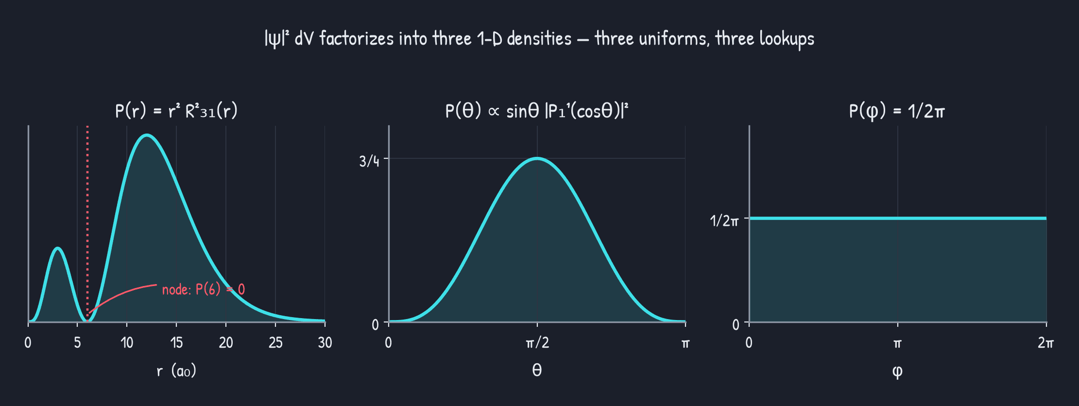
Notice that to produce these graphs, we fill in the factors that are specific to the 3p orbital (n = 3, l = 1, |m| = 1). Then because the PDFs evaluate distances, we vary r, θ, φ and get back the probability that the particle is at that distance when measured.
Converting to 3D Catersian
In order to draw the density map though, we need to produce 3D Cartesian coords (x,y,z) and a probability (w) that the electron is measured at that point:
Here's the first example of a kernel doing the above conversion, for now note only the lines with comments. You can click the link to go to the code on github.
parts/alias-method/src/alias_sample.cuh:10-40 @ alias-method
__global__ void SampleAliasKernel(const AliasBin *radial, int n_radial,
                                          const AliasBin *theta, int n_theta,
                                          curandStateXORWOW_t *states, float *x,
                                          float *y, float *z, float *density, float *r,
                                          float *theta_out, float *phi,
                                          PackedXyzw *packed,
                                          int n, int principal, int l, int m_abs,
                                          float radial_norm, float y_norm) {
            const int i = static_cast<int>(blockIdx.x * blockDim.x + threadIdx.x);
            if (i >= n) {
                return;
            }
            curandStateXORWOW_t rng = states[i]; //hmmm....
            // This is the part we are omitting
            //_________
            const DrawnSample s =
                    DrawAliasSample<Linear>(&rng, radial, n_radial, theta, n_theta, principal,
                                            l, m_abs, radial_norm, y_norm);
            //_________

            states[i] = rng;                    //hmmm!!!!
             // one 16-byte store; what visualization and verification want
            if constexpr (Packed) {
                packed[i] = PackedXyzw{s.x, s.y, s.z, s.density};
            } else {
						// structure-of-arrays: four 4-byte stores
                x[i] = s.x;
                y[i] = s.y;
                z[i] = s.z;
                density[i] = s.density;
            }
            if (r != nullptr) {                     // verify path only
                r[i] = s.r;
                theta_out[i] = s.theta;
                phi[i] = s.phi;
            }
        }
SIDE NOTE (Click):A few notes here: 1. In practice the kernel has ~0 divergence. The first if check verifies we have valid data, which we mostly will. The next 2 checks verify values that will remain constant for the whole of grid time. This can be verified in Nsight. 2. I usually write kernels that allow for packed paths because on the host it can be terribly difficult to allocate packed addresses with correct tilts for device compute. Despite this, they are extremely important for coalesced memory actions. Coalesced operations are just as important for input and output memory operations as Siboehm’s article stresses. Notice how this kernel puts an aggressive amount of effort into making sure that both IN and OUT paths have coalescing.
A few notes here:
- In practice the kernel has ~0 divergence. The first if check verifies we have valid data, which we mostly will. The next 2 checks verify values that will remain constant for the whole of grid time. This can be verified in Nsight.
- I usually write kernels that allow for packed paths because on the host it can be terribly difficult to allocate packed addresses with correct tilts for device compute. Despite this, they are extremely important for coalesced memory actions. Coalesced operations are just as important for input and output memory operations as Siboehm’s article stresses. Notice how this kernel puts an aggressive amount of effort into making sure that both IN and OUT paths have coalescing.
The first 4 floats (16 bytes) here are sent out as output. Despite knowing this is bandwidth bound, we still really want to keep the number of FLOPs we do down (we can’t risk needing to solve 2 problems at the same time)!
The x,y,z position component is computed directly and makes use of no randomly selected components.
We need to be extremely careful here as a simple implementation like:
float x = sinf(th)*cosf(ph)*r
will generate well over 10 FMAs. This might be necessary if you genuinely need over 7 levels of decimal accuracy and are using full precision. Luckily we don’t, as such we use one of the lovely SPMF path functions that ship with CUDA in math_functions.h. In my kernel the computation is done like this:
parts/naive-cuda/src/device_math.cuh:137-143 @ naive-cuda
__host__ __device__ inline void DeviceSinCosFast(float a, float* s, float* c) {
#ifdef __CUDA_ARCH__
  __sincosf(a, s, c);
#else
  sincosf(a, s, c);
#endif
}
Counting the FMA-like operations in SASS gives us 9 FMAs at this level:
4 for sincos(th) and sincos(ph)
plus 1 for radius*sin_th (used twice)
plus 4 for the other multiplications
Then we need to solve for the probability of finding the electron at that point:
In our kernel this follows a highly divergent path:
sample.density = qmc::naive::WavefunctionDensity(n, l, m_abs, radius, th,
                                                 radial_norm, y_norm)
The complexity here comes from the associated Legendre function, which has to climb to the right (l, m). This is how we do it.
parts/naive-cuda/src/device_math.cuh:58-90 @ naive-cuda
template <class Real>
__host__ __device__ inline Real AssociatedLegendrePositiveM(int l, int m,
                                                            Real x) {
  Real pmm = Real(1);
  if (m > 0) {
   // seed P_m^m = (-1)^m (2m-1)!! (1-x²)^{m/2}
    Real somx2 = (Real(1) - x) * (Real(1) + x);
    if (somx2 < Real(0)) {
      somx2 = Real(0);
    }
    somx2 = sqrt(somx2);
    Real fact = Real(1);
    for (int j = 1; j <= m; ++j) {
      pmm *= -fact * somx2;
      fact += Real(2);
    }
  }
  if (l == m) {
    return pmm;
  }
   // P_{m+1}^m
  Real pm1m = x * (Real(2) * static_cast<Real>(m) + Real(1)) * pmm;
  if (l == m + 1) {
    return pm1m;
  }
  Real pll = pm1m;
  for (int ll = m + 2; ll <= l; ++ll) {
   // climb l at fixed m: the stable direction
    pll = ((Real(2) * static_cast<Real>(ll) - Real(1)) * x * pm1m -
           (static_cast<Real>(ll) + static_cast<Real>(m) - Real(1)) * pmm) /
          static_cast<Real>(ll - m);
    pmm = pm1m;
    pm1m = pll;
  }
  return pm1m;
}
We use templates because we want to account for both the float and double paths. But note the number of times we appear to diverge. In reality, the quantum numbers are the same for every thread in one launch, as such we see no scheduler level divergence. The table below lists the approximate operation counts for the pieces of the density:
piece | operations |
|---|---|
| 1 |
|
|
Laguerre |
|
Legendre |
|
square both factors, fold in the host-precomputed constant | 4 mul |
The normalization ($\mathcal{N}_{nl}^{2}$ and the factorial ratio in $|Y_{lm}|^2$) is a single constant for every orbital and it is computed in the host in FP64. The Legendre seed ($\sqrt{1-\cos^2\theta} = \sin\theta$) uses only values we have already computed from the coordinate change so its parameters are in our registers (essentially free).
So given the range of FLOP counts we expect, we allow for an average.
The ground state $(1,0,0)$ is about 10 FMAs + one SFU exp per sample = 11 FMAs.
The deepest orbital in this version is $(5,0,0)$ which has a degree-4 radial polynomial which uses ~25 FMAs.
Adding the 9 for the position, one sample costs somewhere between 20 and 34 FMAs depending on (n, l, m). It is tempting at this point to start optimizing the compute path: pre-evaluate the recurrences into a table, or fuse the squares. It is certainly possible. But let’s pause for a minute and look at the two lines I marked in the kernel:
curandStateXORWOW_t rng = states[i]; // We are loading a random state....
// This is the part we are omitting
//_________
const DrawnSample s =
DrawAliasSample<Linear>(&rng, radial, n_radial, theta, n_theta, principal,
l, m_abs, radial_norm, y_norm);
//_________
states[i] = rng;                    //We are putting back our state? Why?
The physics starts to fight us
curandStateXORWOW_t is CUDA's default way to have a parallel random state but it is still the most expensive part of our pipeline. Say we want to sample a random state 1024 times in parallel. This can be complex because we certainly don’t want to force a thread to randomize numbers before it does its compute, the process of generating random numbers is itself expensive. If we can’t do it as part of the compute loop, we need a much better way to do it.
curand_init(…) allows us to pass in a seed, subsequence, offset and state. The state here is a pointer to a device allocated array of curandStateXORWOW. The function handles the process of creating the random struct and storing it in the location. curand_init is itself a device function, meaning you don’t need to spin CPU cycles computing something of a magnitude you already decided the CPU couldn’t do.
parts/naive-cuda/src/xorwow_setup.cu:12-18 @ naive-cuda
__global__ void SetupXorwowKernel(curandStateXORWOW_t* states,
                                  unsigned long long seed, int n) {
  const int i = static_cast<int>(blockIdx.x * blockDim.x + threadIdx.x);
  if (i < n) {
    curand_init(seed, static_cast<unsigned long long>(i), 0, &states[i]);
  }
}
Here we generate a collection of states using curand_init. Then, in the actual draw kernel we use the states, ensuring to update each used state to represent the fact that it has been used a certain number of times. The convenience we get here is worth it, say we wanted a random uniform float from our random state:
QUALIFIERS float curand_uniform(curandStateXORWOW_t *state)
{
    return _curand_uniform(curand(state));
}
Incredibly easy, but right now the next thread might need to reuse this same uniform so CUDA does exactly the work needed to make sure that it gets a random value we can accept:
QUALIFIERS unsigned int curand(curandStateXORWOW_t *state)
{
    unsigned int t;
    t = (state->v[0] ^ (state->v[0] >> 2));
    state->v[0] = state->v[1];
    state->v[1] = state->v[2];
    state->v[2] = state->v[3];
    state->v[3] = state->v[4];
    state->v[4] = (state->v[4] ^ (state->v[4] <<4)) ^ (t ^ (t << 1));
    state->d += 362437;
    return state->v[4] + state->d;
}
How big is that random state?
// Extracted from curand_kernel.h
struct curandStateXORWOW {
    unsigned int d, v[5];                 // 4 + (5*4) = 24 bytes
    int boxmuller_flag;                   // 4 bytes
    int boxmuller_flag_double;            // 4 bytes
    float boxmuller_extra;                // 4 bytes
    // padding for double                 // 4 bytes
    double boxmuller_extra_double;        // 8 bytes
};
                                          // 48 bytes
It’s 48 bytes, and we are moving it twice in and out of DRAM per sample (96 bytes).
To summarize our bandwidth per sample:

The DRAM bill of one sample, by kernel generation. In kernels 1 through 6 the random state is 86% of the bytes and none of the answer.
My Nvidia RTX 2070 has an FP32 rate of about 3.75 T FMA/s with a DRAM copy bandwidth of 305 GB/s. As such the ridge of the roofline sits at:
On the other hand, our kernel is currently doing:
That is forty to seventy times under the ridge. Following this, we know that we are writing a system that is tens of times more memory bound than compute bound.
Even assuming we got the state traffic to zero, 34 FMA over 16 bytes is 2.1 FMA/B and roughly six times under our ridge. We have an exceptionally bandwidth bound problem here and a lot of work to do, with that said here is our roofline graph:
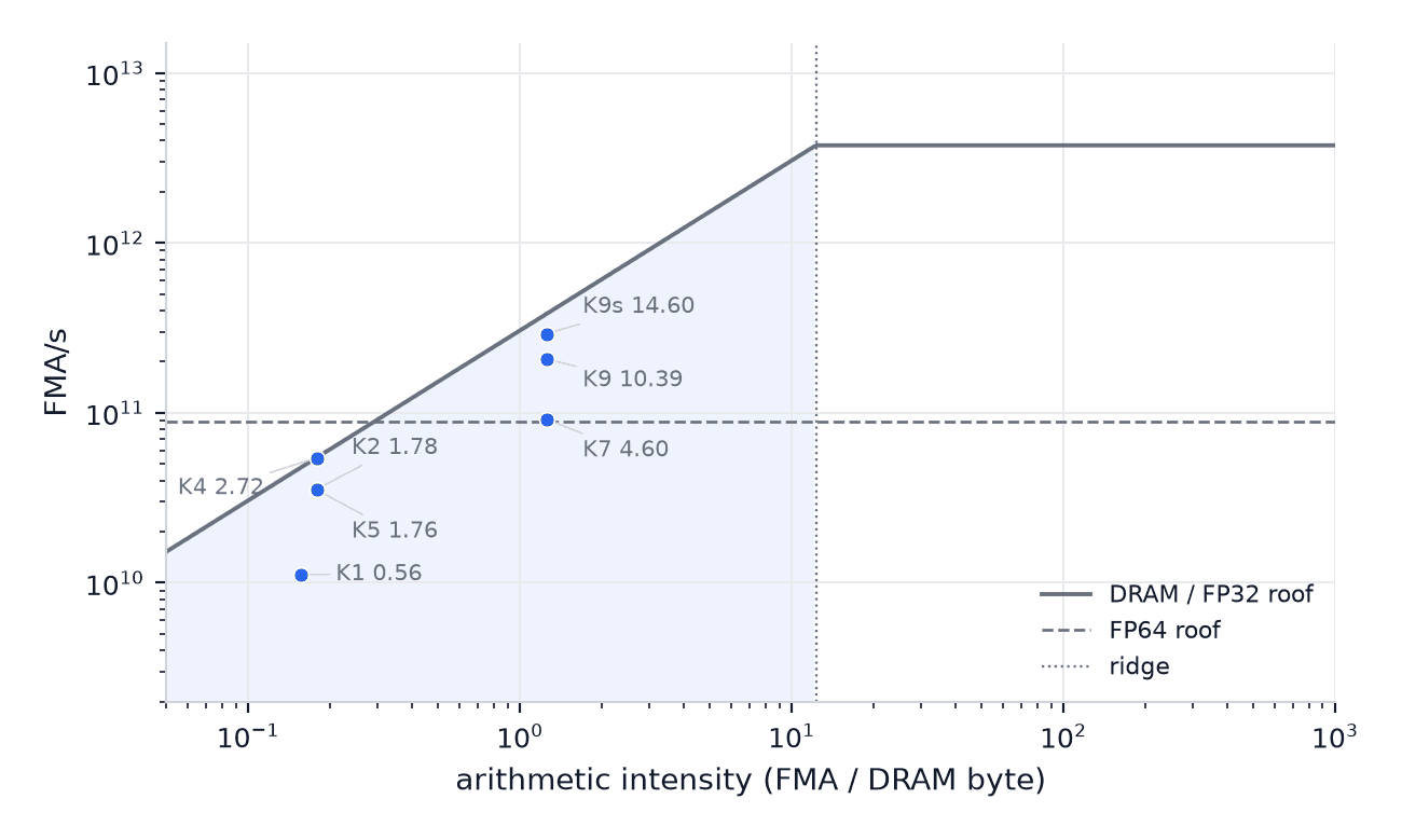
Our roofline. We are going to create 9 kernels in this article and I’ve tried to model their locations in the graph to give you an idea of what changes to expect at each level.
SIDE NOTE (Click):The dependency bug in roofline
Because Williams’ model gives us the upper bound of our kernel compute as min (peak compute, bandwidth * arithmetic intensity). In our case, we can clearly see the kernel is below both of those limits and the model genuinely can’t tell us much. The constraint in this case is latency, we have a load-store queue that’s full but while the roofline calculations tell us where to look, they don’t point to the exact component of the system to check. Nsight Compute gives us a more useful insight. When both Compute (SM) throughput and DRAM throughput are low it says: “this typically indicates latency issues”.
We will build three kernels before reaching kernel 4, which is the first time we shall touch the roofline and get some feedback from it. This is in no form some criticism of the roofline as much as it is a praise of the simplicity of the pattern, it tells you what to aim for and when to stop.
Nsight Compute shows us two special stalls here:
- Long Scoreboard is for when a warp waits for long to get data from L1TEX (essentially a potentially DRAM memory load is taking long)
- LG Throttle even worse, is for when warps are unable to issue load commands because the load/store unit queue is full.
SIDE NOTE (Click):Considering occupancy
For this we can consider Little’s Law. A 4-cycle FMA on Turing’s four schedulers per SM can be hidden using 16 resident warps. However if we wanted to hide a DRAM miss we would need to hide 400 cycles, and would need to issue 1600 warps but a single SM can only host 32 at a time. So we can’t really aim to use any kind of concurrency here; we would instead stress the device and see stream stalling.
The importance and difficulty of accuracy
One more section before we start the kernel implementations. For a physics system like this the importance of being accurate can’t be overstated.
SIDE NOTE (Click):My first development of this kernel in particular adopted a common error in this compute path that has silently spread around the internet I think mostly undetected. The most common implementation of this visualizer samples the density using the build-CDF-then-invert path. This normally inherits 3 common errors. One is a stale CDF table, that ends up using the same static set for all orbitals. The 2nd is Bin-edge quantization. The third is getting the wrong sign of m (which appears correct in renders because m travels as m^2 which erases the sign error). I might touch more on these errors in the physics focused follow up to this article as understanding why they happen and pass initial analysis requires a deep dive into derivation and right now we are eager to start implementing kernels.
My first development of this kernel in particular adopted a common error in this compute path that has silently spread around the internet I think mostly undetected. The most common implementation of this visualizer samples the density using the build-CDF-then-invert path. This normally inherits 3 common errors. One is a stale CDF table, that ends up using the same static set for all orbitals. The 2nd is Bin-edge quantization. The third is getting the wrong sign of m (which appears correct in renders because m travels as m^2 which erases the sign error). I might touch more on these errors in the physics focused follow up to this article as understanding why they happen and pass initial analysis requires a deep dive into derivation and right now we are eager to start implementing kernels.
Because of this the usual CPU side FP64 verifications that nvidia recommends are even more important for us. I’ll use the rest of this section to run through them quickly. The sensitive orbitals for the error variables for this computation are: {(1,0,0), (2,0,0), (2,1,1), (3,1,−1), (4,2,0), (5,0,0)}.
These orbitals show special properties that differ easily if the GPU makes a mistake so I use them to build a CPU side verification process that samples 10 million times for each orbital and verifies the following:
Moments. The sample means of r, r² and 1/r must land within five standard errors of the closed forms from Bethe and Salpeter: ⟨r⟩ = ½(3n² − l(l+1)), ⟨r²⟩ = (n²/2)(5n² + 1 − 3l(l+1)), ⟨1/r⟩ = 1/n². These are the analytic oracle; nothing in the code path can fake them.
Kolmogorov–Smirnov on the radial and polar marginals against the reference CDF at ten times the table resolution, D ≤ 5×10⁻⁴.
χ² on 128 radial, 64 polar and 36 azimuthal bins, pass if χ² ≤ k + 5√(2k) (206.7, 119.1, 76.8). The azimuthal one is the φ-uniformity test.
The node window. 40 fine bins on r ∈ [4.5, 7.5] for the orbital (3,1,−1), whose radial density has a zero at r = 6. Pass ceiling 83.2. This is the only test in the suite that catches the bug in kernel 4, and it exists because I planted it in the hypothesis before writing kernel 4.
Determinism. The same (seed, sample index) must produce identical bits on re-draw, and, from kernel 7 on, on any launch geometry.
Note that the CPU path allows FP64 (double) space accuracy. The reason for this is that we genuinely extract very small numbers in terms of both density and space (often < 3 DPs). At that level, it becomes hard to meet the noise floor for the Monte Carlo we are doing: the relative five-sigma half-width on ⟨r⟩ for the ground state is 2.89/√N, which is 9.1×10⁻⁴ at 10⁷ samples and 9.1×10⁻⁵ at 10⁹. FLT_EPSILON is 1.2×10⁻⁷.
Our compute needs to be able to detect an FP32 rounding since we need to make sure that rounding is unbiased as rounding should not cancel out and form important components of the final float draw path. But to do that we need N > ~10^15. That requirement is the key reason our CDF, alias and normalization constant tables are built on the CPU using FP64. The float path would bias every draw in the same way and wreck our accuracy. These errors are often not caught in many online implementations where a developer naively issues a float since this is a floating value. This is usually fine for visualization (especially of simple states) but produces a broken layer that might be used in future layers of an actual physics engine.

Maximum relative error of FP32 radial recurrence against FP64 per (n, l) on a 200-point grid out to r=10n^2. The two outliers are at the nodes, where the numerator is ~0 and relative error is meaningless. You can take a much closer look at the experimental data in parts/naive-cuda/experiments/fp32_vs_fp64.json on the naive-cuda branch.
You can see here that the relative error of the FP32 recurrences is 5×10⁻⁷ and well below the band. The actual device weights, checked on 10⁷ samples with |w| > 10⁻⁸, come in at a maximum relative error of 7.7×10⁻⁵ against the FP64 reference, still under the 10⁹-sample band. The intrinsics are also inside it: __expf is specified at 2 + ⌊1.17·|x|⌋ ULP, which is 25 ULP at r = 20, about 3×10⁻⁶ relative. So float is licensed, not by a flag flip, but by arithmetic.
As a quick reference beyond accuracy, the CPU compute runs at 2.1 million and 15.1 million samples per second for the single-threaded and 16-thread variants respectively. The path uses super efficient libm calls which deserve a whole exploration on their own.
So here is what we carry into the kernels. One sample costs 20 to 34 FMAs and 112 bytes of DRAM traffic, 96 of them random state, and the ridge sits at 12.3 FMA/B, so every kernel below is bandwidth bound long before it is compute bound. The verification suite tells us whether a fast kernel is also a correct one, and the CPU numbers are the referee to beat. I built nine kernels on the way to the final number. The ones that moved it get a section; the ones that didn’t get a side note where they happened, because what they taught still matters.
Kernel 1:
The first implementation is a natural direct port of the CPU solution, you can check out the entire implementation in parts/naive-cuda/src starting in sample_double.cu:73.
Tracking the flow you’ll see:
LaunchSampleFp64 → SampleFp64Kernel → DrawOne → 2 InvertCdf calls.
We are stepping the InvertCdf calls as they are the primary bandwidth steps. Note though that the other parts make use of the state we load as discussed before to produce the x,y,z,w products as discussed earlier:parts/naive-cuda/src/device_math.cu: 207-219 It’s worth getting acquainted with that shape as we proceed. As noted earlier though we need the state to change after we observe it.
parts/naive-cuda/src/device_math.cuh:15-33 @ naive-cuda
template <class Real>
__host__ __device__ inline Real InvertCdf(const Real* nodes, const Real* cdf,
                                          int n, Real u) {
  if (u <= cdf[0]) { return nodes[0]; }
  if (u >= cdf[n - 1]) { return nodes[n - 1]; }
  const Real* it = cuda::std::lower_bound(cdf, cdf + n, u);   // 12 dependent loads
  const int i = static_cast<int>(it - cdf);
  if (i == 0) { return nodes[0]; }
  const Real c0 = cdf[i - 1];
  const Real c1 = cdf[i];
  const Real t = (c1 > c0) ? (u - c0) / (c1 - c0) : Real(0);
  return nodes[i - 1] + t * (nodes[i] - nodes[i - 1]);        // lerp inside the bin
}
Given this, let’s run the test and see what we get:
0.560 Gsamples/s (14.3 ms per 8M samples). Well this is surprisingly fast and drastically outperforms my card’s measured DRAM bandwidth. So to figure out what’s going on we go to Nsight:
The tables are not in DRAM. 4096 + 2048 doubles of CDF plus the same of nodes is 96 KiB, and my system die has 4 MiB of L2. With a hit rate 84% which also resulted in DRAM throughput of 19% of peak.
The binary search also does not diverge. Branch efficiency is 100%, 0.01 divergent branches per warp. The compiler predicates
lower_bound, so all 32 lanes walk 12 steps in lockstep and the cost is the dependent chain of 12 loads, each of which pulls a 32-byte sector to use 8 bytes of it (68% of sectors wasted).Compute throughput 85%. Nsight’s reports: the FP64 pipe “over-utilized and likely a performance bottleneck”, 53% of FP64 peak issue. That rate implies about ~160 FP64-equivalent ops per sample.
As expected we have 65 cycles between issued instructions per warp, 43 of them long-scoreboard stalls on L1TEX.
Taking a look at parts/naive-cuda/src/device_math.cu: 190 Note the range we are drawing from: curandStateXORWOW_t . As discussed we need this range to be generated before we start sampling, you can see that being done in parts/naive-cuda/src/xorwow_setup.cu:12 using the curand_init function as discussed that drops them directly into DRAM. In the Systems timeline this generation takes up about 60% of GPU time - it’s mostly a compute step and as per our calculated roofs we don’t need to try and optimize it.
Kernel 2: FP32
As per Nsight’s report we can make some easy wins. We simply change the compute path to use floats:
LaunchSampleFp64 → SampleFp64Kernel → DrawOne → 2 InvertCdf calls
To use floats we maintain table generation in doubles and cast them to floats during the sample process. This is rather easy to do because InvertCdf and DrawOne are already template functions.
SIDE NOTE (Click):Templating, inline device function is one of those things I do almost out of habit and it’s great practice. It helps a lot with variant testing and predictable stacks. Creating monolith kernel functions that compute everything in a single large block is neither great to read nor run.
Templating, inline device function is one of those things I do almost out of habit and it’s great practice. It helps a lot with variant testing and predictable stacks. Creating monolith kernel functions that compute everything in a single large block is neither great to read nor run.
Measuring this cheap change:
1.776 Gsamples/s. FP32 over FP64 gives us 3.2×, not the 42× the pipes would give, because Kernel 2 is not on a compute pipe at all:
We are using 31% compute throughput, DRAM throughput 52%, and 3% of FP32 peak. The busiest compute pipe is the integer ALU at 31%, doing address arithmetic for the search.
LG throttle at 54% of a 30-cycle issue gap, then long scoreboard at 31%. Hmm… the warps are neither waiting on compute nor DRAM. They are essentially waiting for permission to issue DRAM loads.
Occupancy 95%, 49 registers, branch efficiency 100% (note this), 78% of fetched sectors unused.
With that we are finally hitting a roofline (Figure 5). Looking at these specs we can revisit the use of intrinsics mentioned earlier and as you can see it only shows results in compute only because we are entirely bandwidth bound and it cuts instructions on a device pipe that only ever ran at ~3%. We leave it in here though as it can still come in handy when we start computing multiple particles later.
SIDE NOTE (Click):Kernel 3: shared memory didn't help much
Staging the CDF tables produced 1.37 Gsamples/s which was slower than kernel 2 at every threads/block setting. The shared search meant lanes collided in the same banks (7.1-way conflicts), occupancy halved and instructions went from 7.5 to 36 million per million samples. A dependent chain of loads does not care which SRAM it chains through.
Shared memory did deliver wins in kernel 9 later on.
Data: `parts/inverse-table/results/shared_cdf.json` on inverse-table.
Kernel 4: replacing the search with a table
Using inversion here is essentially asking “which bin contains u?” twelve times. We can save these queries by asking the inverse. If we store F^-1 at K uniformly spaced values of u, then a draw can be done as one multiply, one truncation and one lerp between neighbors. It’s now essentially O(1) and branch-free.
parts/inverse-table/src/lookup.cuh:10-21 @ inverse-table
__device__ inline float QuantileLerp(const float* table, int k, float u) {
  const float x = u * static_cast<float>(k - 1);
  int idx = static_cast<int>(x);
  if (idx < 0) { idx = 0; }
  if (idx > k - 2) { idx = k - 2; }
  const float frac = x - static_cast<float>(idx);
  return table[idx] + frac * (table[idx + 1] - table[idx]);
}
We build tables on the host in FP64 by inverting the fine CDF at 4096 radial and 2048 polar knots before casting to float.
Now we measure 2.720 Gsamples/s, a 53% improvement. For the first time as well, Nsight agrees with the roofline. DRAM throughput 85.7% (300 GB/s against the 305 measured roof), compute 11%, 5% of FP32 peak, 7.5 million instructions per million samples against kernel 3’s 36 million. Williams’ model finally has something to say, and what it says is that the XORWOW state is the bill. No kernel that still carries that 48-byte object can beat 2.7 Gsamples/s on this card. That is a bandwidth fact.
In hindsight, this is not a statement about our correctness. So I’d like us to take sometime on this.
Looking back at Figure 2, the radial density of (3,1) has a zero at r = 6. Every orbital with n-l-1 ≥ 1 has these radial nodes, spheres on which the electron is never found. In the CDF, a zero of density is a flat: F(r) stops increasing across the node. In the inverse, F^-1(u), a flat becomes a jump: an infinitesimal step in u carries r from one side of the node to the other.
Now put a uniformly spaced table on that. Two neighboring knots $u_i$ and $u_{i+1}$ straddle the jump, and QuantileLerp draws a straight line between $r(u_i)$ ≈ 5.75 and $r(u_{i+1})$ ≈ 6.39. Every u in that interval, one in 4095 of all draws, lands on the chord, strictly inside the region where the density is zero. The kernel manufactures electrons where the physics forbids them, at a rate that is small, deterministic, and invisible to almost every test you would think to run.

Left: the CDF of (3,1) with the flat at r = 6. Right: the quantile F⁻¹(u) around the node, with the 4096-knot table’s chord drawn across the jump. Everything on that chord is a sample the electron cannot produce.
The moment tests pass; a few thousand samples out of ten million do not move ⟨r⟩. KS passes; a leak of mass ε moves the KS statistic by at most ε, and ε here is 2.4×10⁻⁴ against a threshold of 5×10⁻⁴. The coarse 128-bin χ² passes, because no coarse bin is empty enough to notice. The 40-bin node window is the only gate that fires, and it fires with χ² = 11,572 against a ceiling of 83. In the hypothesis I had written that this would happen, and I had written that the fix I was tempted by, a bigger table, would not work:

Node-window χ² for (3,1,−1) against table size. The lerp table shrinks the hole like 1/K and does not reach the ceiling until K = 65536, sixteen times the memory. The “snap” variant (do not interpolate across a flagged interval, snap to the nearer knot) helps at small K and is worse than lerp at large K. Data: parts/inverse-table/experiments/node_trap.json on branch inverse-table, 10⁶ samples.
The 1/K law is exactly what you expect: one straddling interval, 1/(K−1) of the mass. Snapping to the nearer knot halves the leak and then, at very large K, starts to bias the neighboring bins the other way. Neither is a fix. The lesson I want to state in general terms: inversion by tabulation is exact between knots only where the quantile is smooth, and a node makes it discontinuous. The interpolation error bounds in the literature (Hörmann and Leydold’s numerical inversion work, for one) assume a C² quantile, and a node breaks the assumption rather than the bound.
The fastest kernel of the first six had this bug and a benchmark table would have hidden it.
SIDE NOTE (Click):Kernel 5: the alias method
The node trap’s fix is not a bigger table. Walker and Vose’s alias method picks a bin with a fair die and a biased coin, and a bin with zero mass can never be kept: the node window went from χ² = 11,572 to 37. It cost throughput, 1.76 Gsamples/s, because two data-dependent 24-byte records per sample are uncoalesced loads and seven uniforms add instructions (11.0 million per million samples against kernel 4’s 7.5). It is the draw we counted at the start, and every later kernel keeps it.
Kernel 6 tried textbook layout moves on top: float4 against SoA output (1.759 against 1.760 Gsamples/s) and a split draw/weight pipeline (1.51). Neither touched the 96 bytes of state that were the bill. Data: `parts/alias-method/results` on alias-method.
Kernel 7: Eliminating the random state
Salmon, Moraes, Dror and Shaw’s 2011 paper (title: “Parallel Random Numbers: As Easy as 1, 2, 3”) discussed a parallel random number generator as a function function you call: x_n = b_k(n), a keyed bijection of a counter. The n-th random block is computed from n directly. So we get no state to load, store, or initialize with a 182 ms skip-ahead kernel, and the same (n, key) gives the same bits on any thread and any launch geometry, which is a property the verification suite can test for.

A counter-based random generator is a pure function of the sample index.
Their Philox4x32-10 generator is ten rounds of a Feistel-like mixing step built from 32-bit multiply-high/low and XOR, about 100 integer operations for 128 bits of output, and it passes the BigCrush battery. It is also about fifty lines to to implement:
harness/rng/philox.h:35-62,79-87 @ endgame
QMC_HOST_DEVICE inline Philox4x32Ctr Philox4x32Round(Philox4x32Ctr ctr, Philox4x32Key key) {
  std::uint32_t lo0 = 0, lo1 = 0;
  const std::uint32_t hi0 = MulHiLo32(kPhiloxM0, ctr.v[0], &lo0);   // 0xD2511F53
  const std::uint32_t hi1 = MulHiLo32(kPhiloxM1, ctr.v[2], &lo1);   // 0xCD9E8D57
  Philox4x32Ctr out;
  out.v[0] = hi1 ^ ctr.v[1] ^ key.v[0];
  out.v[1] = lo1;
  out.v[2] = hi0 ^ ctr.v[3] ^ key.v[1];
  out.v[3] = lo0;
  return out;
}
QMC_HOST_DEVICE inline Philox4x32Ctr Philox4x32TenRounds(Philox4x32Ctr ctr, Philox4x32Key key) {
  for (int round = 0; round < 10; ++round) {
    ctr = Philox4x32Round(ctr, key);
    key = BumpKey(key);                 // Weyl sequence: += 0x9E3779B9, 0xBB67AE85
  }
  return ctr;
}
QMC_HOST_DEVICE inline Philox4x32Ctr MakeCounter(std::uint32_t sample_index, std::uint32_t draw_slot) {
  Philox4x32Ctr ctr;
  ctr.v[0] = sample_index;  ctr.v[1] = draw_slot;  ctr.v[2] = 0;  ctr.v[3] = 0;
  return ctr;
}
The counter is (sample index, draw slot): one Philox call yields four uniforms, the alias draw needs seven, so each sample makes two calls at slots 0 and 1 and wastes one lane (parts/endgame/src/philox_draw.cuh:22-37 @ endgame).
The key is the 64-bit seed. The sample kernel loses two lines and a parameter:
parts/endgame/src/philox_sample.cu:22-29 @ endgame
const int i = static_cast<int>(blockIdx.x * blockDim.x + threadIdx.x);
if (i >= n) { return; }
const qmc::alias::DrawnSample s =
    DrawPhiloxSample(static_cast<std::uint32_t>(i), seed, radial, n_radial,
                     theta, n_theta, principal, l, m_abs, radial_norm, y_norm);
StoreSample(s, i, packed, x, y, z, density, r, theta_out, phi)
Measured: 4.60 Gsamples/s. The setup kernel is gone from the timeline; the profiler shows the sample kernel at 100% of GPU time. DRAM throughput fell from 54% to 16%, 57 GB/s, and L2 hit rate went to 99.9%. The 96 bytes were real DRAM traffic, and now they are not.
But 4.60 is four times under the 16-byte roof, and the stall that was supposed to drain did not: LG throttle at 71% of the issue gap, 83% of fetched sectors unused, 4.2 of every 32 bytes per sector consumed, L1TEX throughput at 96%. Deleting the state deleted the bytes but the scatter is a latency problem.
SIDE NOTE (Click):Kernel 8: Volkov’s trade, tried
With occupancy at 94%, I gave each thread S independent samples so it would have S gathers in flight, and predicted 8.5 Gsamples/s. Every S > 1 was slower: the best cell was S = 1, which is kernel 7 again (4.59), and occupancy fell to 69%. Each of those samples issues the same two uncoalesced gathers into the same full queue, and more in-flight loads only lengthen the line. It lost again per process on the global packed version of kernel 9 (9.45 at S = 2 against 10.39). Data: `parts/endgame/results/philox_ilp.json` on endgame.
Kernel 9: the return of shared memory
Looking at the SASS for kernel 7 (cuobjdump -sass), the one load looks like this:
LDG.E.CONSTANT.SYS R25, [R10]          ; radial prob
LDG.E.CONSTANT.SYS R24, [R8]           ; theta  prob
@!P0 LDG.E.CONSTANT.SYS R23, [R10+0x4] ; radial alias (predicated on the coin)
@!P1 LDG.E.CONSTANT.SYS R7,  [R8+0x4]  ; theta  alias
LDG.E.CONSTANT.SYS R23, [R28+0x8]      ; lo     (axis A)
LDG.E.CONSTANT.SYS R24, [R28+0xc]      ; width  (axis A)
LDG.E.CONSTANT.SYS R27, [R28+0x10]     ; y0     (axis A)
LDG.E.CONSTANT.SYS R0,  [R28+0x14]     ; y1     (axis A)
LDG.E.CONSTANT.SYS R19, [R6+0x8]       ; lo     (axis B)
LDG.E.CONSTANT.SYS R22, [R6+0xc]       ; width  (axis B)
LDG.E.CONSTANT.SYS R25, [R6+0x10]      ; y0     (axis B)
LDG.E.CONSTANT.SYS R26, [R6+0x14]      ; y1     (axis B)
@P0 STG.E.128.SYS [R2], R24            ; the 16 B output
Twelve scalar four-byte gathers per sample. Not two 24-byte loads. A struct with no alignas has an alignment of 4, and nvcc is not allowed to emit a 64- or 128-bit load for it even though 24·j happens to be 8-byte aligned for every j; the compiler works from the declared alignment, not from arithmetic it cannot prove. Each of those twelve loads is a divergent access that pulls a 32-byte sector to consume 4 bytes of it. That is the “4.2 bytes per sector” line from kernel 7’s profile, explained to the byte, and it is why the load queue never drained: every sample was twelve entries in it.

The 24-byte record as the compiler saw it, and the split, aligned records that replaced it.
The fix is to give the fair-die probe exactly the record Vose’s algorithm needs and nothing else, and to declare its alignment:
parts/packed-records/src/sampler.h:20-32 @ packed-records
struct alignas(8) AliasDraw {
  float prob = 0.0f;
  std::uint32_t alias = 0;
};
static_assert(sizeof(AliasDraw) == 8, "AliasDraw must be one 64-bit load");

struct alignas(8) BinUniform {   // within-bin geometry, read only for the winner
  float lo = 0.0f;
  float width = 0.0f;
}
The table build copies the kernel 5 values into the three arrays without recomputing anything, so kernel 9 is bitwise comparable to kernel 7. The draw becomes one LDG.E.64 per axis, and the interior fields one more aligned load for the winning bin only: four vector gathers instead of twelve scalar ones.
Measured, draw arrays in shared memory: 14.60 Gsamples/s. 1.41× over the global version, 1.72× over my prediction, well past the line.
parts/packed-records/src/packed_sample.cu:46-63 @ packed-records
extern __shared__ __align__(8) unsigned char smem_raw[];
AliasDraw* s_radial = reinterpret_cast<AliasDraw*>(smem_raw);
AliasDraw* s_theta = s_radial + n_radial;
for (int t = threadIdx.x; t < n_radial + n_theta; t += blockDim.x) {
  s_radial[t] = (t < n_radial) ? radial_draw[t] : theta_draw[t - n_radial];
}
__syncthreads();
const int tid = blockIdx.x * blockDim.x + threadIdx.x;
const int stride = blockDim.x * gridDim.x;
for (int i = tid; i < n; i += stride) {   // grid-stride: pay the staging once per block
  const DrawnSample s = DrawPackedSample<BinUniform>(i, seed, s_radial, radial_bin, n_radial,
                                                     s_theta, theta_bin, n_theta, ...);
  StoreSample(s, i, ...);
}
The model was wrong in exactly the way the falsification clause anticipated. The SRAM is shared; the access machinery is not. A random 8-byte LDS across 32 lanes does cost bank-conflict replays (Nsight counts 68% excess shared wavefronts, a 6.3-way conflict), but a shared load skips the tag stage and never enters the load/store unit’s global queue. That queue was the constraint since kernel 2, and the shared path simply is not in it. Warp cycles per issued instruction fell from 14.8 to 6.3; IPC rose from 1.9 to 2.5; and for the first time three pipes sit in the busy band at once, L1TEX 95%, compute 62%, DRAM 55%. The occupancy tax I priced is real (49.6%) and irrelevant.
So why did shared memory lose in kernel 3 and win here? Kernel 3 moved a dependent chain of twelve loads into shared memory, and a chain is latency-bound wherever it lives; the relocation bought conflicts and divergence and cost occupancy. Kernel 9 moves two independent gathers, whose problem was queue pressure, not latency, onto a path that has no such queue. Same SRAM, opposite result, and the difference is which resource the loads were actually contending for. The kernel 3 lesson “don’t chase shared memory” does not generalize from one access pattern to the other, and I had generalized it.
The remaining uncoalesced global traffic (58% of sectors) is the interior-geometry gathers. They are the next target if there ever is one, and the answer to “why not shared too” is that they add 49 KB to the footprint and the block would not fit.

The shared-memory kernel across the six verification orbitals. Data: parts/packed-records/results/orbital_sweep.json on branch packed-records.
Across the orbital matrix, from the 11-FMA ground state to the 25-FMA (5,0,0), throughput spreads by 17.5%. The recurrence trip counts are compute, and compute is still not the roof; it has just stopped being nothing. That slope is the door into Act II, where the per-sample math grows by an order of magnitude and the ridge is finally in play.
The third axis: watts
One more prediction on the kernel 9 hypothesis sheet was boring: “64M samples versus 8M, same rate, ±3%”. It measured −42%, and the day it took to find out why is the most transferable thing in this article if you benchmark on a laptop.
The chain of evidence, in the order I found it. An identical 8M cell repeated six times in one process decays 10.4 → 9.9 → 8.2 → 6.8 and never recovers; every fresh process reads 10.4 again. A sweep over output footprint is flat at 14.8 to 24M samples (366 MiB) and falls off a cliff to 8.7 at 64M. That looked exactly like TLB reach, and I believed it for several hours, until cuRAND writing a full 1 GiB of uniforms turned out to be flat at 272 GB/s, which a pure store stream would not be if the cliff were address translation. Then the rep arrays killed the footprint story too: the first 64M repetition runs at 4.22 ms, 15.2 Gsamples/s, full speed, and the twentieth takes 10.2 ms. The slowdown is progressive within a run. Nsight, which replays kernels at base clock with gaps between them, sees the 8M and 64M cells as identical per cycle. Finally nvidia-smi sampled in the middle of a repetition: SM clock 750 MHz, 95.6 W, throttle reason 0x4, SW_POWER_CAP.

Repetition time relative to the first repetition, for the kernel 9 variants at 8M and 64M samples. Short repetitions with normal gaps never trip the governor; long back-to-back ones do, and the clock lock is a ceiling that does not hold. Data: rep arrays in parts/packed-records/results/*.json on branch packed-records; note that the 64M files were captured with the lock flag reading false.
This kernel pulls about 95 W at 1500 MHz. The 80 W budget is enforced by averaging over a window of a second or two; a 0.5 ms repetition with harness gaps between it never fills the window, and a 4 ms repetition, twenty times back to back, fills it and gets the clock halved. The lock I set with nvidia-smi -lgc is a maximum, not a floor. The “TLB cliff” at 400 MiB was the point at which one repetition got long enough to trip the governor before it ended.
Two consequences. First, an instrument rule that now governs every number in this article: one process per cell, and n ≤ 8M for anything in a series. The kernel 8 launch sweep, which was run in-process, carries that caveat retroactively (its ordering survived spot checks; its later cells are pessimistic). Second, an honest framing of the headline: 14.6 Gsamples/s is the locked-clock burst rate, and it is the right number to compare with kernels 1 through 8 because they are all sub-15 ms bursts under the same window. Sustained, on this 80 W part, the same kernel does about 8.5 to 9 Gsamples/s, bounded by watts rather than by any pipe Nsight can see. The roofline has a third axis on mobile silicon, and no profiler draws it.
Verdict

The whole climb, with the three referee lines: the idiomatic Thrust + cuRAND pipeline, cuRAND’s own raw-uniform bandwidth expressed in 16-byte samples, and the measured copy roof. Every bar is 8M samples of (1,0,0), median of 20, clocks locked at 1500 MHz, one process per cell. Files and commits in the table at the top.
A few things I want to note at this point for this nature of computational problem:
Itemize the random state. In a sampling kernel the generator’s storage is a byte term, often the dominant one, and it is invisible in every FLOP count. Counter-based generation (Philox, or anything in the Random123 family) deletes it, gives you bitwise reproducibility across launch geometries for free, and costs about 100 integer ops that Turing co-issues next to the float work.
Read the SASS for your record loads. A struct you did not
alignasis a scalar load per field. The compiler will not vectorize on arithmetic it cannot prove.The profiler’s sentence “latency issues” means the roofline is off duty. Look at LG throttle versus long scoreboard. A full queue and a slow load are different diseases with different cures, and shared memory cures one of them.
Plant the correctness failure before you optimize. The node window existed because the hypothesis said kernel 4 would leak, and kernel 4 leaked. Nothing in the standard statistical kit (moments, KS, coarse χ²) would have caught it, and the benchmark table would have crowned the wrong kernel.
On a laptop, the clock lock is a ceiling. One process per cell, short cells, and log the clock inside every repetition.
And the sentence the drop was built to earn, now with the arithmetic behind it: sampling a full hydrogen orbital costs about as much as generating the random bits alone.
Preparing for act II
One of the hardest problems I’ve had to deal with is simulating more than 2 particles. With two electrons the density |ψ(r₁, r₂)|² does not factorize into one-dimensional pieces. We have to use a Markov chain instead: walkers that propose a move, evaluate the trial wave function, and accept or reject. The computational concepts involved are still really important though, so I'll carry them into that implementation.
Further reading/useful references
The knowledge for construction of these pipelines comes from a wide range of sources. I’ll list here, and hopefully add more along the way, my favorite ones grouped by what they contribute.
Random numbers.
Salmon, Moraes, Dror and Shaw, Parallel Random Numbers: As Easy as 1, 2, 3, SC’11 (paper, code). The single most important reference here; the argument for counter-based generation is in the first four pages.
Marsaglia, Xorshift RNGs, J. Stat. Softw. 2003 (link) for what XORWOW’s 24 real bytes are doing.
The cuRAND guide, device API and testing sections, for the 48-byte struct and the BigCrush results.
Sampling.
Keith Schwarz, Darts, Dice, and Coins (essay) is the clearest explanation of the alias method that exists;
Walker 1977 (TOMS) and Vose 1991 (TSE) for attribution. Devroye, Non-Uniform Random Variate Generation, 1986, free at his site, chapters II and III, for inversion as the master idea and the error of tabulating it.
Hörmann and Leydold, Continuous Random Variate Generation by Fast Numerical Inversion, TOMACS 2003 (link) for the smoothness assumption the node breaks.
The machine.
Boehm’s matmul worklog, one the best guides for solving compute bound problems in CUDA.
Volkov, Better Performance at Lower Occupancy, GTC 2010 (slides). Williams, Waterman and Patterson, Roofline, CACM 2009 (link).
The Nsight Compute Kernel Profiling Guide for the stall-reason vocabulary, the CUDA Best Practices Guide §10.2.1 for 32-byte sectors, the Programming Guide’s intrinsic ULP table for
__expfand__sincosf, and the Turing tuning guide for INT32 co-issue.
The physics.
Griffiths and Schroeter, Introduction to Quantum Mechanics, 3rd ed., chapter 4, for the separation into R(r)Y(θ,φ).
Bethe and Salpeter, Quantum Mechanics of One- and Two-Electron Atoms, 1957, §3, for the analytic moments the verify suite uses as its oracle.
DLMF §18.9 and §14.10 for the Laguerre and Legendre recurrences and which direction they are stable in.
Numerical Recipes §6.8 (2nd ed.) for
plgndr, the shape my Legendre routine follows.Hoarau and Rayez, Comment about the use of Monte-Carlo methodology for the representation of atomic electronic densities.
Eur. J. Phys. 2016 (arXiv), on the Jacobian mistake in published orbital pictures; it is the one classic error the tests in this article did not need to plant, because the factorization in Figure 2 has the r² and sin θ built in.
Orbital visualizers that show this simulation. kavang.com/atom (source, CDF inversion, the same method as kernel 1); Evanescence (source, accept-reject); Quantum Atom Simulator (rejection sampling); Falstad’s viewer and the Wolfram demonstration (volumetric, no sampling); The plate at the top of this article is from Electron, by n, 2018, Wikipedia (wikipedia.org), Creative Commons License.
Share this post:
Optimizing Quantum Monte Carlo Sampling in CUDA
September 7, 2026
Motivation
We are blessed to have a good library of resources that teach computation of dense elements operators in CUDA and form the great foundation for us to analyze complex compute bound GPU problems and optimize them.
However, many kernels that run computational physics demand that we deal with bandwidth bound compute. This article aims to contribute a thought process for discovering and attacking such problems (along with the relevant data) by choosing a particularly difficult but common example: Quantum Monte Carlo sampling.
Hydrogen atomic orbitals at different energy levels. The more opaque areas are where one is most likely to find an electron at any given time. From Electron, by n, 2018, Wikipedia (wikipedia.org). Creative Commons License.
We wish to determine a hydrogen atom’s electron density probability and optimize the two step compute pipeline involved in doing so. As we progress we find the requirements of quantum computation fight us constantly: we fix the bottleneck caused by the randomization machinery that takes up 86% of the available memory bandwidth by itself. At the end of our development we rendered this sample:
SIDE NOTE (Click):Note here the red dotted line, in that region a particle sampled in the (3, 1, -1) state can’t be present. As such sampling there is a waste of compute? But wait even having the information needed to sample there is a waste of memory bandwidth.
Note here the red dotted line, in that region a particle sampled in the (3, 1, -1) state can’t be present. As such sampling there is a waste of compute? But wait even having the information needed to sample there is a waste of memory bandwidth.
The contribution of this piece will remain mainly computational. To achieve I will avoid extensive physics derivations and only include those that contribute to understanding the compute and accuracy requirements. A later article will dive into how the decisions that take us from wave equations to C++ lines are made I will link it here when it's ready. For now, let’s talk compute:
Our end goal is to produce a cloud of positions that are sampled randomly each with a density that tells us the likelihood that the electron is present when a measurement is taken at that position. Quantum states are truly random however, and change on observation, this feature will cause of most our headaches.
The compute pipeline
The compute pipeline involves 2 stages. To get an overview of the cause of the bandwidth problem, let's go over both briefly.
First we must compute three independent probability densities:
These three PDFs solve for three different properties of the electron, we need all three before we can start solving 3D Cartesian position. For example the hydrogen 3p orbital can be plotted as these three PDFs in it's three coordinates:
Notice that to produce these graphs, we fill in the factors that are specific to the 3p orbital (n = 3, l = 1, |m| = 1). Then because the PDFs evaluate distances, we vary r, θ, φ and get back the probability that the particle is at that distance when measured.
Converting to 3D Catersian
In order to draw the density map though, we need to produce 3D Cartesian coords (x,y,z) and a probability (w) that the electron is measured at that point:
Here's the first example of a kernel doing the above conversion, for now note only the lines with comments. You can click the link to go to the code on github.
parts/alias-method/src/alias_sample.cuh:10-40 @ alias-method
__global__ void SampleAliasKernel(const AliasBin *radial, int n_radial,
                                          const AliasBin *theta, int n_theta,
                                          curandStateXORWOW_t *states, float *x,
                                          float *y, float *z, float *density, float *r,
                                          float *theta_out, float *phi,
                                          PackedXyzw *packed,
                                          int n, int principal, int l, int m_abs,
                                          float radial_norm, float y_norm) {
            const int i = static_cast<int>(blockIdx.x * blockDim.x + threadIdx.x);
            if (i >= n) {
                return;
            }
            curandStateXORWOW_t rng = states[i]; //hmmm....
            // This is the part we are omitting
            //_________
            const DrawnSample s =
                    DrawAliasSample<Linear>(&rng, radial, n_radial, theta, n_theta, principal,
                                            l, m_abs, radial_norm, y_norm);
            //_________

            states[i] = rng;                    //hmmm!!!!
             // one 16-byte store; what visualization and verification want
            if constexpr (Packed) {
                packed[i] = PackedXyzw{s.x, s.y, s.z, s.density};
            } else {
						// structure-of-arrays: four 4-byte stores
                x[i] = s.x;
                y[i] = s.y;
                z[i] = s.z;
                density[i] = s.density;
            }
            if (r != nullptr) {                     // verify path only
                r[i] = s.r;
                theta_out[i] = s.theta;
                phi[i] = s.phi;
            }
        }
SIDE NOTE (Click):A few notes here: 1. In practice the kernel has ~0 divergence. The first if check verifies we have valid data, which we mostly will. The next 2 checks verify values that will remain constant for the whole of grid time. This can be verified in Nsight. 2. I usually write kernels that allow for packed paths because on the host it can be terribly difficult to allocate packed addresses with correct tilts for device compute. Despite this, they are extremely important for coalesced memory actions. Coalesced operations are just as important for input and output memory operations as Siboehm’s article stresses. Notice how this kernel puts an aggressive amount of effort into making sure that both IN and OUT paths have coalescing.
A few notes here:
- In practice the kernel has ~0 divergence. The first if check verifies we have valid data, which we mostly will. The next 2 checks verify values that will remain constant for the whole of grid time. This can be verified in Nsight.
- I usually write kernels that allow for packed paths because on the host it can be terribly difficult to allocate packed addresses with correct tilts for device compute. Despite this, they are extremely important for coalesced memory actions. Coalesced operations are just as important for input and output memory operations as Siboehm’s article stresses. Notice how this kernel puts an aggressive amount of effort into making sure that both IN and OUT paths have coalescing.
The first 4 floats (16 bytes) here are sent out as output. Despite knowing this is bandwidth bound, we still really want to keep the number of FLOPs we do down (we can’t risk needing to solve 2 problems at the same time)!
The x,y,z position component is computed directly and makes use of no randomly selected components.
We need to be extremely careful here as a simple implementation like:
float x = sinf(th)*cosf(ph)*r
will generate well over 10 FMAs. This might be necessary if you genuinely need over 7 levels of decimal accuracy and are using full precision. Luckily we don’t, as such we use one of the lovely SPMF path functions that ship with CUDA in math_functions.h. In my kernel the computation is done like this:
parts/naive-cuda/src/device_math.cuh:137-143 @ naive-cuda
__host__ __device__ inline void DeviceSinCosFast(float a, float* s, float* c) {
#ifdef __CUDA_ARCH__
  __sincosf(a, s, c);
#else
  sincosf(a, s, c);
#endif
}
Counting the FMA-like operations in SASS gives us 9 FMAs at this level:
4 for sincos(th) and sincos(ph)
plus 1 for radius*sin_th (used twice)
plus 4 for the other multiplications
Then we need to solve for the probability of finding the electron at that point:
In our kernel this follows a highly divergent path:
sample.density = qmc::naive::WavefunctionDensity(n, l, m_abs, radius, th,
                                                 radial_norm, y_norm)
The complexity here comes from the associated Legendre function, which has to climb to the right (l, m). This is how we do it.
parts/naive-cuda/src/device_math.cuh:58-90 @ naive-cuda
template <class Real>
__host__ __device__ inline Real AssociatedLegendrePositiveM(int l, int m,
                                                            Real x) {
  Real pmm = Real(1);
  if (m > 0) {
   // seed P_m^m = (-1)^m (2m-1)!! (1-x²)^{m/2}
    Real somx2 = (Real(1) - x) * (Real(1) + x);
    if (somx2 < Real(0)) {
      somx2 = Real(0);
    }
    somx2 = sqrt(somx2);
    Real fact = Real(1);
    for (int j = 1; j <= m; ++j) {
      pmm *= -fact * somx2;
      fact += Real(2);
    }
  }
  if (l == m) {
    return pmm;
  }
   // P_{m+1}^m
  Real pm1m = x * (Real(2) * static_cast<Real>(m) + Real(1)) * pmm;
  if (l == m + 1) {
    return pm1m;
  }
  Real pll = pm1m;
  for (int ll = m + 2; ll <= l; ++ll) {
   // climb l at fixed m: the stable direction
    pll = ((Real(2) * static_cast<Real>(ll) - Real(1)) * x * pm1m -
           (static_cast<Real>(ll) + static_cast<Real>(m) - Real(1)) * pmm) /
          static_cast<Real>(ll - m);
    pmm = pm1m;
    pm1m = pll;
  }
  return pm1m;
}
We use templates because we want to account for both the float and double paths. But note the number of times we appear to diverge. In reality, the quantum numbers are the same for every thread in one launch, as such we see no scheduler level divergence. The table below lists the approximate operation counts for the pieces of the density:
piece | operations |
|---|---|
| 1 |
|
|
Laguerre |
|
Legendre |
|
square both factors, fold in the host-precomputed constant | 4 mul |
The normalization ($\mathcal{N}_{nl}^{2}$ and the factorial ratio in $|Y_{lm}|^2$) is a single constant for every orbital and it is computed in the host in FP64. The Legendre seed ($\sqrt{1-\cos^2\theta} = \sin\theta$) uses only values we have already computed from the coordinate change so its parameters are in our registers (essentially free).
So given the range of FLOP counts we expect, we allow for an average.
The ground state $(1,0,0)$ is about 10 FMAs + one SFU exp per sample = 11 FMAs.
The deepest orbital in this version is $(5,0,0)$ which has a degree-4 radial polynomial which uses ~25 FMAs.
Adding the 9 for the position, one sample costs somewhere between 20 and 34 FMAs depending on (n, l, m). It is tempting at this point to start optimizing the compute path: pre-evaluate the recurrences into a table, or fuse the squares. It is certainly possible. But let’s pause for a minute and look at the two lines I marked in the kernel:
curandStateXORWOW_t rng = states[i]; // We are loading a random state....
// This is the part we are omitting
//_________
const DrawnSample s =
DrawAliasSample<Linear>(&rng, radial, n_radial, theta, n_theta, principal,
l, m_abs, radial_norm, y_norm);
//_________
states[i] = rng;                    //We are putting back our state? Why?
The physics starts to fight us
curandStateXORWOW_t is CUDA's default way to have a parallel random state but it is still the most expensive part of our pipeline. Say we want to sample a random state 1024 times in parallel. This can be complex because we certainly don’t want to force a thread to randomize numbers before it does its compute, the process of generating random numbers is itself expensive. If we can’t do it as part of the compute loop, we need a much better way to do it.
curand_init(…) allows us to pass in a seed, subsequence, offset and state. The state here is a pointer to a device allocated array of curandStateXORWOW. The function handles the process of creating the random struct and storing it in the location. curand_init is itself a device function, meaning you don’t need to spin CPU cycles computing something of a magnitude you already decided the CPU couldn’t do.
parts/naive-cuda/src/xorwow_setup.cu:12-18 @ naive-cuda
__global__ void SetupXorwowKernel(curandStateXORWOW_t* states,
                                  unsigned long long seed, int n) {
  const int i = static_cast<int>(blockIdx.x * blockDim.x + threadIdx.x);
  if (i < n) {
    curand_init(seed, static_cast<unsigned long long>(i), 0, &states[i]);
  }
}
Here we generate a collection of states using curand_init. Then, in the actual draw kernel we use the states, ensuring to update each used state to represent the fact that it has been used a certain number of times. The convenience we get here is worth it, say we wanted a random uniform float from our random state:
QUALIFIERS float curand_uniform(curandStateXORWOW_t *state)
{
    return _curand_uniform(curand(state));
}
Incredibly easy, but right now the next thread might need to reuse this same uniform so CUDA does exactly the work needed to make sure that it gets a random value we can accept:
QUALIFIERS unsigned int curand(curandStateXORWOW_t *state)
{
    unsigned int t;
    t = (state->v[0] ^ (state->v[0] >> 2));
    state->v[0] = state->v[1];
    state->v[1] = state->v[2];
    state->v[2] = state->v[3];
    state->v[3] = state->v[4];
    state->v[4] = (state->v[4] ^ (state->v[4] <<4)) ^ (t ^ (t << 1));
    state->d += 362437;
    return state->v[4] + state->d;
}
How big is that random state?
// Extracted from curand_kernel.h
struct curandStateXORWOW {
    unsigned int d, v[5];                 // 4 + (5*4) = 24 bytes
    int boxmuller_flag;                   // 4 bytes
    int boxmuller_flag_double;            // 4 bytes
    float boxmuller_extra;                // 4 bytes
    // padding for double                 // 4 bytes
    double boxmuller_extra_double;        // 8 bytes
};
                                          // 48 bytes
It’s 48 bytes, and we are moving it twice in and out of DRAM per sample (96 bytes).
To summarize our bandwidth per sample:
The DRAM bill of one sample, by kernel generation. In kernels 1 through 6 the random state is 86% of the bytes and none of the answer.
My Nvidia RTX 2070 has an FP32 rate of about 3.75 T FMA/s with a DRAM copy bandwidth of 305 GB/s. As such the ridge of the roofline sits at:
On the other hand, our kernel is currently doing:
That is forty to seventy times under the ridge. Following this, we know that we are writing a system that is tens of times more memory bound than compute bound.
Even assuming we got the state traffic to zero, 34 FMA over 16 bytes is 2.1 FMA/B and roughly six times under our ridge. We have an exceptionally bandwidth bound problem here and a lot of work to do, with that said here is our roofline graph:
Our roofline. We are going to create 9 kernels in this article and I’ve tried to model their locations in the graph to give you an idea of what changes to expect at each level.
SIDE NOTE (Click):The dependency bug in roofline
Because Williams’ model gives us the upper bound of our kernel compute as min (peak compute, bandwidth * arithmetic intensity). In our case, we can clearly see the kernel is below both of those limits and the model genuinely can’t tell us much. The constraint in this case is latency, we have a load-store queue that’s full but while the roofline calculations tell us where to look, they don’t point to the exact component of the system to check. Nsight Compute gives us a more useful insight. When both Compute (SM) throughput and DRAM throughput are low it says: “this typically indicates latency issues”.
We will build three kernels before reaching kernel 4, which is the first time we shall touch the roofline and get some feedback from it. This is in no form some criticism of the roofline as much as it is a praise of the simplicity of the pattern, it tells you what to aim for and when to stop.
Nsight Compute shows us two special stalls here:
- Long Scoreboard is for when a warp waits for long to get data from L1TEX (essentially a potentially DRAM memory load is taking long)
- LG Throttle even worse, is for when warps are unable to issue load commands because the load/store unit queue is full.
SIDE NOTE (Click):Considering occupancy
For this we can consider Little’s Law. A 4-cycle FMA on Turing’s four schedulers per SM can be hidden using 16 resident warps. However if we wanted to hide a DRAM miss we would need to hide 400 cycles, and would need to issue 1600 warps but a single SM can only host 32 at a time. So we can’t really aim to use any kind of concurrency here; we would instead stress the device and see stream stalling.
The importance and difficulty of accuracy
One more section before we start the kernel implementations. For a physics system like this the importance of being accurate can’t be overstated.
SIDE NOTE (Click):My first development of this kernel in particular adopted a common error in this compute path that has silently spread around the internet I think mostly undetected. The most common implementation of this visualizer samples the density using the build-CDF-then-invert path. This normally inherits 3 common errors. One is a stale CDF table, that ends up using the same static set for all orbitals. The 2nd is Bin-edge quantization. The third is getting the wrong sign of m (which appears correct in renders because m travels as m^2 which erases the sign error). I might touch more on these errors in the physics focused follow up to this article as understanding why they happen and pass initial analysis requires a deep dive into derivation and right now we are eager to start implementing kernels.
My first development of this kernel in particular adopted a common error in this compute path that has silently spread around the internet I think mostly undetected. The most common implementation of this visualizer samples the density using the build-CDF-then-invert path. This normally inherits 3 common errors. One is a stale CDF table, that ends up using the same static set for all orbitals. The 2nd is Bin-edge quantization. The third is getting the wrong sign of m (which appears correct in renders because m travels as m^2 which erases the sign error). I might touch more on these errors in the physics focused follow up to this article as understanding why they happen and pass initial analysis requires a deep dive into derivation and right now we are eager to start implementing kernels.
Because of this the usual CPU side FP64 verifications that nvidia recommends are even more important for us. I’ll use the rest of this section to run through them quickly. The sensitive orbitals for the error variables for this computation are: {(1,0,0), (2,0,0), (2,1,1), (3,1,−1), (4,2,0), (5,0,0)}.
These orbitals show special properties that differ easily if the GPU makes a mistake so I use them to build a CPU side verification process that samples 10 million times for each orbital and verifies the following:
Moments. The sample means of r, r² and 1/r must land within five standard errors of the closed forms from Bethe and Salpeter: ⟨r⟩ = ½(3n² − l(l+1)), ⟨r²⟩ = (n²/2)(5n² + 1 − 3l(l+1)), ⟨1/r⟩ = 1/n². These are the analytic oracle; nothing in the code path can fake them.
Kolmogorov–Smirnov on the radial and polar marginals against the reference CDF at ten times the table resolution, D ≤ 5×10⁻⁴.
χ² on 128 radial, 64 polar and 36 azimuthal bins, pass if χ² ≤ k + 5√(2k) (206.7, 119.1, 76.8). The azimuthal one is the φ-uniformity test.
The node window. 40 fine bins on r ∈ [4.5, 7.5] for the orbital (3,1,−1), whose radial density has a zero at r = 6. Pass ceiling 83.2. This is the only test in the suite that catches the bug in kernel 4, and it exists because I planted it in the hypothesis before writing kernel 4.
Determinism. The same (seed, sample index) must produce identical bits on re-draw, and, from kernel 7 on, on any launch geometry.
Note that the CPU path allows FP64 (double) space accuracy. The reason for this is that we genuinely extract very small numbers in terms of both density and space (often < 3 DPs). At that level, it becomes hard to meet the noise floor for the Monte Carlo we are doing: the relative five-sigma half-width on ⟨r⟩ for the ground state is 2.89/√N, which is 9.1×10⁻⁴ at 10⁷ samples and 9.1×10⁻⁵ at 10⁹. FLT_EPSILON is 1.2×10⁻⁷.
Our compute needs to be able to detect an FP32 rounding since we need to make sure that rounding is unbiased as rounding should not cancel out and form important components of the final float draw path. But to do that we need N > ~10^15. That requirement is the key reason our CDF, alias and normalization constant tables are built on the CPU using FP64. The float path would bias every draw in the same way and wreck our accuracy. These errors are often not caught in many online implementations where a developer naively issues a float since this is a floating value. This is usually fine for visualization (especially of simple states) but produces a broken layer that might be used in future layers of an actual physics engine.
Maximum relative error of FP32 radial recurrence against FP64 per (n, l) on a 200-point grid out to r=10n^2. The two outliers are at the nodes, where the numerator is ~0 and relative error is meaningless. You can take a much closer look at the experimental data in parts/naive-cuda/experiments/fp32_vs_fp64.json on the naive-cuda branch.
You can see here that the relative error of the FP32 recurrences is 5×10⁻⁷ and well below the band. The actual device weights, checked on 10⁷ samples with |w| > 10⁻⁸, come in at a maximum relative error of 7.7×10⁻⁵ against the FP64 reference, still under the 10⁹-sample band. The intrinsics are also inside it: __expf is specified at 2 + ⌊1.17·|x|⌋ ULP, which is 25 ULP at r = 20, about 3×10⁻⁶ relative. So float is licensed, not by a flag flip, but by arithmetic.
As a quick reference beyond accuracy, the CPU compute runs at 2.1 million and 15.1 million samples per second for the single-threaded and 16-thread variants respectively. The path uses super efficient libm calls which deserve a whole exploration on their own.
So here is what we carry into the kernels. One sample costs 20 to 34 FMAs and 112 bytes of DRAM traffic, 96 of them random state, and the ridge sits at 12.3 FMA/B, so every kernel below is bandwidth bound long before it is compute bound. The verification suite tells us whether a fast kernel is also a correct one, and the CPU numbers are the referee to beat. I built nine kernels on the way to the final number. The ones that moved it get a section; the ones that didn’t get a side note where they happened, because what they taught still matters.
Kernel 1:
The first implementation is a natural direct port of the CPU solution, you can check out the entire implementation in parts/naive-cuda/src starting in sample_double.cu:73.
Tracking the flow you’ll see:
LaunchSampleFp64 → SampleFp64Kernel → DrawOne → 2 InvertCdf calls.
We are stepping the InvertCdf calls as they are the primary bandwidth steps. Note though that the other parts make use of the state we load as discussed before to produce the x,y,z,w products as discussed earlier:parts/naive-cuda/src/device_math.cu: 207-219 It’s worth getting acquainted with that shape as we proceed. As noted earlier though we need the state to change after we observe it.
parts/naive-cuda/src/device_math.cuh:15-33 @ naive-cuda
template <class Real>
__host__ __device__ inline Real InvertCdf(const Real* nodes, const Real* cdf,
                                          int n, Real u) {
  if (u <= cdf[0]) { return nodes[0]; }
  if (u >= cdf[n - 1]) { return nodes[n - 1]; }
  const Real* it = cuda::std::lower_bound(cdf, cdf + n, u);   // 12 dependent loads
  const int i = static_cast<int>(it - cdf);
  if (i == 0) { return nodes[0]; }
  const Real c0 = cdf[i - 1];
  const Real c1 = cdf[i];
  const Real t = (c1 > c0) ? (u - c0) / (c1 - c0) : Real(0);
  return nodes[i - 1] + t * (nodes[i] - nodes[i - 1]);        // lerp inside the bin
}
Given this, let’s run the test and see what we get:
0.560 Gsamples/s (14.3 ms per 8M samples). Well this is surprisingly fast and drastically outperforms my card’s measured DRAM bandwidth. So to figure out what’s going on we go to Nsight:
The tables are not in DRAM. 4096 + 2048 doubles of CDF plus the same of nodes is 96 KiB, and my system die has 4 MiB of L2. With a hit rate 84% which also resulted in DRAM throughput of 19% of peak.
The binary search also does not diverge. Branch efficiency is 100%, 0.01 divergent branches per warp. The compiler predicates
lower_bound, so all 32 lanes walk 12 steps in lockstep and the cost is the dependent chain of 12 loads, each of which pulls a 32-byte sector to use 8 bytes of it (68% of sectors wasted).Compute throughput 85%. Nsight’s reports: the FP64 pipe “over-utilized and likely a performance bottleneck”, 53% of FP64 peak issue. That rate implies about ~160 FP64-equivalent ops per sample.
As expected we have 65 cycles between issued instructions per warp, 43 of them long-scoreboard stalls on L1TEX.
Taking a look at parts/naive-cuda/src/device_math.cu: 190 Note the range we are drawing from: curandStateXORWOW_t . As discussed we need this range to be generated before we start sampling, you can see that being done in parts/naive-cuda/src/xorwow_setup.cu:12 using the curand_init function as discussed that drops them directly into DRAM. In the Systems timeline this generation takes up about 60% of GPU time - it’s mostly a compute step and as per our calculated roofs we don’t need to try and optimize it.
Kernel 2: FP32
As per Nsight’s report we can make some easy wins. We simply change the compute path to use floats:
LaunchSampleFp64 → SampleFp64Kernel → DrawOne → 2 InvertCdf calls
To use floats we maintain table generation in doubles and cast them to floats during the sample process. This is rather easy to do because InvertCdf and DrawOne are already template functions.
SIDE NOTE (Click):Templating, inline device function is one of those things I do almost out of habit and it’s great practice. It helps a lot with variant testing and predictable stacks. Creating monolith kernel functions that compute everything in a single large block is neither great to read nor run.
Templating, inline device function is one of those things I do almost out of habit and it’s great practice. It helps a lot with variant testing and predictable stacks. Creating monolith kernel functions that compute everything in a single large block is neither great to read nor run.
Measuring this cheap change:
1.776 Gsamples/s. FP32 over FP64 gives us 3.2×, not the 42× the pipes would give, because Kernel 2 is not on a compute pipe at all:
We are using 31% compute throughput, DRAM throughput 52%, and 3% of FP32 peak. The busiest compute pipe is the integer ALU at 31%, doing address arithmetic for the search.
LG throttle at 54% of a 30-cycle issue gap, then long scoreboard at 31%. Hmm… the warps are neither waiting on compute nor DRAM. They are essentially waiting for permission to issue DRAM loads.
Occupancy 95%, 49 registers, branch efficiency 100% (note this), 78% of fetched sectors unused.
With that we are finally hitting a roofline (Figure 5). Looking at these specs we can revisit the use of intrinsics mentioned earlier and as you can see it only shows results in compute only because we are entirely bandwidth bound and it cuts instructions on a device pipe that only ever ran at ~3%. We leave it in here though as it can still come in handy when we start computing multiple particles later.
SIDE NOTE (Click):Kernel 3: shared memory didn't help much
Staging the CDF tables produced 1.37 Gsamples/s which was slower than kernel 2 at every threads/block setting. The shared search meant lanes collided in the same banks (7.1-way conflicts), occupancy halved and instructions went from 7.5 to 36 million per million samples. A dependent chain of loads does not care which SRAM it chains through.
Shared memory did deliver wins in kernel 9 later on.
Data: `parts/inverse-table/results/shared_cdf.json` on inverse-table.
Kernel 4: replacing the search with a table
Using inversion here is essentially asking “which bin contains u?” twelve times. We can save these queries by asking the inverse. If we store F^-1 at K uniformly spaced values of u, then a draw can be done as one multiply, one truncation and one lerp between neighbors. It’s now essentially O(1) and branch-free.
parts/inverse-table/src/lookup.cuh:10-21 @ inverse-table
__device__ inline float QuantileLerp(const float* table, int k, float u) {
  const float x = u * static_cast<float>(k - 1);
  int idx = static_cast<int>(x);
  if (idx < 0) { idx = 0; }
  if (idx > k - 2) { idx = k - 2; }
  const float frac = x - static_cast<float>(idx);
  return table[idx] + frac * (table[idx + 1] - table[idx]);
}
We build tables on the host in FP64 by inverting the fine CDF at 4096 radial and 2048 polar knots before casting to float.
Now we measure 2.720 Gsamples/s, a 53% improvement. For the first time as well, Nsight agrees with the roofline. DRAM throughput 85.7% (300 GB/s against the 305 measured roof), compute 11%, 5% of FP32 peak, 7.5 million instructions per million samples against kernel 3’s 36 million. Williams’ model finally has something to say, and what it says is that the XORWOW state is the bill. No kernel that still carries that 48-byte object can beat 2.7 Gsamples/s on this card. That is a bandwidth fact.
In hindsight, this is not a statement about our correctness. So I’d like us to take sometime on this.
Looking back at Figure 2, the radial density of (3,1) has a zero at r = 6. Every orbital with n-l-1 ≥ 1 has these radial nodes, spheres on which the electron is never found. In the CDF, a zero of density is a flat: F(r) stops increasing across the node. In the inverse, F^-1(u), a flat becomes a jump: an infinitesimal step in u carries r from one side of the node to the other.
Now put a uniformly spaced table on that. Two neighboring knots $u_i$ and $u_{i+1}$ straddle the jump, and QuantileLerp draws a straight line between $r(u_i)$ ≈ 5.75 and $r(u_{i+1})$ ≈ 6.39. Every u in that interval, one in 4095 of all draws, lands on the chord, strictly inside the region where the density is zero. The kernel manufactures electrons where the physics forbids them, at a rate that is small, deterministic, and invisible to almost every test you would think to run.
Left: the CDF of (3,1) with the flat at r = 6. Right: the quantile F⁻¹(u) around the node, with the 4096-knot table’s chord drawn across the jump. Everything on that chord is a sample the electron cannot produce.
The moment tests pass; a few thousand samples out of ten million do not move ⟨r⟩. KS passes; a leak of mass ε moves the KS statistic by at most ε, and ε here is 2.4×10⁻⁴ against a threshold of 5×10⁻⁴. The coarse 128-bin χ² passes, because no coarse bin is empty enough to notice. The 40-bin node window is the only gate that fires, and it fires with χ² = 11,572 against a ceiling of 83. In the hypothesis I had written that this would happen, and I had written that the fix I was tempted by, a bigger table, would not work:
Node-window χ² for (3,1,−1) against table size. The lerp table shrinks the hole like 1/K and does not reach the ceiling until K = 65536, sixteen times the memory. The “snap” variant (do not interpolate across a flagged interval, snap to the nearer knot) helps at small K and is worse than lerp at large K. Data: parts/inverse-table/experiments/node_trap.json on branch inverse-table, 10⁶ samples.
The 1/K law is exactly what you expect: one straddling interval, 1/(K−1) of the mass. Snapping to the nearer knot halves the leak and then, at very large K, starts to bias the neighboring bins the other way. Neither is a fix. The lesson I want to state in general terms: inversion by tabulation is exact between knots only where the quantile is smooth, and a node makes it discontinuous. The interpolation error bounds in the literature (Hörmann and Leydold’s numerical inversion work, for one) assume a C² quantile, and a node breaks the assumption rather than the bound.
The fastest kernel of the first six had this bug and a benchmark table would have hidden it.
SIDE NOTE (Click):Kernel 5: the alias method
The node trap’s fix is not a bigger table. Walker and Vose’s alias method picks a bin with a fair die and a biased coin, and a bin with zero mass can never be kept: the node window went from χ² = 11,572 to 37. It cost throughput, 1.76 Gsamples/s, because two data-dependent 24-byte records per sample are uncoalesced loads and seven uniforms add instructions (11.0 million per million samples against kernel 4’s 7.5). It is the draw we counted at the start, and every later kernel keeps it.
Kernel 6 tried textbook layout moves on top: float4 against SoA output (1.759 against 1.760 Gsamples/s) and a split draw/weight pipeline (1.51). Neither touched the 96 bytes of state that were the bill. Data: `parts/alias-method/results` on alias-method.
Kernel 7: Eliminating the random state
Salmon, Moraes, Dror and Shaw’s 2011 paper (title: “Parallel Random Numbers: As Easy as 1, 2, 3”) discussed a parallel random number generator as a function function you call: x_n = b_k(n), a keyed bijection of a counter. The n-th random block is computed from n directly. So we get no state to load, store, or initialize with a 182 ms skip-ahead kernel, and the same (n, key) gives the same bits on any thread and any launch geometry, which is a property the verification suite can test for.
A counter-based random generator is a pure function of the sample index.
Their Philox4x32-10 generator is ten rounds of a Feistel-like mixing step built from 32-bit multiply-high/low and XOR, about 100 integer operations for 128 bits of output, and it passes the BigCrush battery. It is also about fifty lines to to implement:
harness/rng/philox.h:35-62,79-87 @ endgame
QMC_HOST_DEVICE inline Philox4x32Ctr Philox4x32Round(Philox4x32Ctr ctr, Philox4x32Key key) {
  std::uint32_t lo0 = 0, lo1 = 0;
  const std::uint32_t hi0 = MulHiLo32(kPhiloxM0, ctr.v[0], &lo0);   // 0xD2511F53
  const std::uint32_t hi1 = MulHiLo32(kPhiloxM1, ctr.v[2], &lo1);   // 0xCD9E8D57
  Philox4x32Ctr out;
  out.v[0] = hi1 ^ ctr.v[1] ^ key.v[0];
  out.v[1] = lo1;
  out.v[2] = hi0 ^ ctr.v[3] ^ key.v[1];
  out.v[3] = lo0;
  return out;
}
QMC_HOST_DEVICE inline Philox4x32Ctr Philox4x32TenRounds(Philox4x32Ctr ctr, Philox4x32Key key) {
  for (int round = 0; round < 10; ++round) {
    ctr = Philox4x32Round(ctr, key);
    key = BumpKey(key);                 // Weyl sequence: += 0x9E3779B9, 0xBB67AE85
  }
  return ctr;
}
QMC_HOST_DEVICE inline Philox4x32Ctr MakeCounter(std::uint32_t sample_index, std::uint32_t draw_slot) {
  Philox4x32Ctr ctr;
  ctr.v[0] = sample_index;  ctr.v[1] = draw_slot;  ctr.v[2] = 0;  ctr.v[3] = 0;
  return ctr;
}
The counter is (sample index, draw slot): one Philox call yields four uniforms, the alias draw needs seven, so each sample makes two calls at slots 0 and 1 and wastes one lane (parts/endgame/src/philox_draw.cuh:22-37 @ endgame).
The key is the 64-bit seed. The sample kernel loses two lines and a parameter:
parts/endgame/src/philox_sample.cu:22-29 @ endgame
const int i = static_cast<int>(blockIdx.x * blockDim.x + threadIdx.x);
if (i >= n) { return; }
const qmc::alias::DrawnSample s =
    DrawPhiloxSample(static_cast<std::uint32_t>(i), seed, radial, n_radial,
                     theta, n_theta, principal, l, m_abs, radial_norm, y_norm);
StoreSample(s, i, packed, x, y, z, density, r, theta_out, phi)
Measured: 4.60 Gsamples/s. The setup kernel is gone from the timeline; the profiler shows the sample kernel at 100% of GPU time. DRAM throughput fell from 54% to 16%, 57 GB/s, and L2 hit rate went to 99.9%. The 96 bytes were real DRAM traffic, and now they are not.
But 4.60 is four times under the 16-byte roof, and the stall that was supposed to drain did not: LG throttle at 71% of the issue gap, 83% of fetched sectors unused, 4.2 of every 32 bytes per sector consumed, L1TEX throughput at 96%. Deleting the state deleted the bytes but the scatter is a latency problem.
SIDE NOTE (Click):Kernel 8: Volkov’s trade, tried
With occupancy at 94%, I gave each thread S independent samples so it would have S gathers in flight, and predicted 8.5 Gsamples/s. Every S > 1 was slower: the best cell was S = 1, which is kernel 7 again (4.59), and occupancy fell to 69%. Each of those samples issues the same two uncoalesced gathers into the same full queue, and more in-flight loads only lengthen the line. It lost again per process on the global packed version of kernel 9 (9.45 at S = 2 against 10.39). Data: `parts/endgame/results/philox_ilp.json` on endgame.
Kernel 9: the return of shared memory
Looking at the SASS for kernel 7 (cuobjdump -sass), the one load looks like this:
LDG.E.CONSTANT.SYS R25, [R10]          ; radial prob
LDG.E.CONSTANT.SYS R24, [R8]           ; theta  prob
@!P0 LDG.E.CONSTANT.SYS R23, [R10+0x4] ; radial alias (predicated on the coin)
@!P1 LDG.E.CONSTANT.SYS R7,  [R8+0x4]  ; theta  alias
LDG.E.CONSTANT.SYS R23, [R28+0x8]      ; lo     (axis A)
LDG.E.CONSTANT.SYS R24, [R28+0xc]      ; width  (axis A)
LDG.E.CONSTANT.SYS R27, [R28+0x10]     ; y0     (axis A)
LDG.E.CONSTANT.SYS R0,  [R28+0x14]     ; y1     (axis A)
LDG.E.CONSTANT.SYS R19, [R6+0x8]       ; lo     (axis B)
LDG.E.CONSTANT.SYS R22, [R6+0xc]       ; width  (axis B)
LDG.E.CONSTANT.SYS R25, [R6+0x10]      ; y0     (axis B)
LDG.E.CONSTANT.SYS R26, [R6+0x14]      ; y1     (axis B)
@P0 STG.E.128.SYS [R2], R24            ; the 16 B output
Twelve scalar four-byte gathers per sample. Not two 24-byte loads. A struct with no alignas has an alignment of 4, and nvcc is not allowed to emit a 64- or 128-bit load for it even though 24·j happens to be 8-byte aligned for every j; the compiler works from the declared alignment, not from arithmetic it cannot prove. Each of those twelve loads is a divergent access that pulls a 32-byte sector to consume 4 bytes of it. That is the “4.2 bytes per sector” line from kernel 7’s profile, explained to the byte, and it is why the load queue never drained: every sample was twelve entries in it.
The 24-byte record as the compiler saw it, and the split, aligned records that replaced it.
The fix is to give the fair-die probe exactly the record Vose’s algorithm needs and nothing else, and to declare its alignment:
parts/packed-records/src/sampler.h:20-32 @ packed-records
struct alignas(8) AliasDraw {
  float prob = 0.0f;
  std::uint32_t alias = 0;
};
static_assert(sizeof(AliasDraw) == 8, "AliasDraw must be one 64-bit load");

struct alignas(8) BinUniform {   // within-bin geometry, read only for the winner
  float lo = 0.0f;
  float width = 0.0f;
}
The table build copies the kernel 5 values into the three arrays without recomputing anything, so kernel 9 is bitwise comparable to kernel 7. The draw becomes one LDG.E.64 per axis, and the interior fields one more aligned load for the winning bin only: four vector gathers instead of twelve scalar ones.
Measured, draw arrays in shared memory: 14.60 Gsamples/s. 1.41× over the global version, 1.72× over my prediction, well past the line.
parts/packed-records/src/packed_sample.cu:46-63 @ packed-records
extern __shared__ __align__(8) unsigned char smem_raw[];
AliasDraw* s_radial = reinterpret_cast<AliasDraw*>(smem_raw);
AliasDraw* s_theta = s_radial + n_radial;
for (int t = threadIdx.x; t < n_radial + n_theta; t += blockDim.x) {
  s_radial[t] = (t < n_radial) ? radial_draw[t] : theta_draw[t - n_radial];
}
__syncthreads();
const int tid = blockIdx.x * blockDim.x + threadIdx.x;
const int stride = blockDim.x * gridDim.x;
for (int i = tid; i < n; i += stride) {   // grid-stride: pay the staging once per block
  const DrawnSample s = DrawPackedSample<BinUniform>(i, seed, s_radial, radial_bin, n_radial,
                                                     s_theta, theta_bin, n_theta, ...);
  StoreSample(s, i, ...);
}
The model was wrong in exactly the way the falsification clause anticipated. The SRAM is shared; the access machinery is not. A random 8-byte LDS across 32 lanes does cost bank-conflict replays (Nsight counts 68% excess shared wavefronts, a 6.3-way conflict), but a shared load skips the tag stage and never enters the load/store unit’s global queue. That queue was the constraint since kernel 2, and the shared path simply is not in it. Warp cycles per issued instruction fell from 14.8 to 6.3; IPC rose from 1.9 to 2.5; and for the first time three pipes sit in the busy band at once, L1TEX 95%, compute 62%, DRAM 55%. The occupancy tax I priced is real (49.6%) and irrelevant.
So why did shared memory lose in kernel 3 and win here? Kernel 3 moved a dependent chain of twelve loads into shared memory, and a chain is latency-bound wherever it lives; the relocation bought conflicts and divergence and cost occupancy. Kernel 9 moves two independent gathers, whose problem was queue pressure, not latency, onto a path that has no such queue. Same SRAM, opposite result, and the difference is which resource the loads were actually contending for. The kernel 3 lesson “don’t chase shared memory” does not generalize from one access pattern to the other, and I had generalized it.
The remaining uncoalesced global traffic (58% of sectors) is the interior-geometry gathers. They are the next target if there ever is one, and the answer to “why not shared too” is that they add 49 KB to the footprint and the block would not fit.
The shared-memory kernel across the six verification orbitals. Data: parts/packed-records/results/orbital_sweep.json on branch packed-records.
Across the orbital matrix, from the 11-FMA ground state to the 25-FMA (5,0,0), throughput spreads by 17.5%. The recurrence trip counts are compute, and compute is still not the roof; it has just stopped being nothing. That slope is the door into Act II, where the per-sample math grows by an order of magnitude and the ridge is finally in play.
The third axis: watts
One more prediction on the kernel 9 hypothesis sheet was boring: “64M samples versus 8M, same rate, ±3%”. It measured −42%, and the day it took to find out why is the most transferable thing in this article if you benchmark on a laptop.
The chain of evidence, in the order I found it. An identical 8M cell repeated six times in one process decays 10.4 → 9.9 → 8.2 → 6.8 and never recovers; every fresh process reads 10.4 again. A sweep over output footprint is flat at 14.8 to 24M samples (366 MiB) and falls off a cliff to 8.7 at 64M. That looked exactly like TLB reach, and I believed it for several hours, until cuRAND writing a full 1 GiB of uniforms turned out to be flat at 272 GB/s, which a pure store stream would not be if the cliff were address translation. Then the rep arrays killed the footprint story too: the first 64M repetition runs at 4.22 ms, 15.2 Gsamples/s, full speed, and the twentieth takes 10.2 ms. The slowdown is progressive within a run. Nsight, which replays kernels at base clock with gaps between them, sees the 8M and 64M cells as identical per cycle. Finally nvidia-smi sampled in the middle of a repetition: SM clock 750 MHz, 95.6 W, throttle reason 0x4, SW_POWER_CAP.
Repetition time relative to the first repetition, for the kernel 9 variants at 8M and 64M samples. Short repetitions with normal gaps never trip the governor; long back-to-back ones do, and the clock lock is a ceiling that does not hold. Data: rep arrays in parts/packed-records/results/*.json on branch packed-records; note that the 64M files were captured with the lock flag reading false.
This kernel pulls about 95 W at 1500 MHz. The 80 W budget is enforced by averaging over a window of a second or two; a 0.5 ms repetition with harness gaps between it never fills the window, and a 4 ms repetition, twenty times back to back, fills it and gets the clock halved. The lock I set with nvidia-smi -lgc is a maximum, not a floor. The “TLB cliff” at 400 MiB was the point at which one repetition got long enough to trip the governor before it ended.
Two consequences. First, an instrument rule that now governs every number in this article: one process per cell, and n ≤ 8M for anything in a series. The kernel 8 launch sweep, which was run in-process, carries that caveat retroactively (its ordering survived spot checks; its later cells are pessimistic). Second, an honest framing of the headline: 14.6 Gsamples/s is the locked-clock burst rate, and it is the right number to compare with kernels 1 through 8 because they are all sub-15 ms bursts under the same window. Sustained, on this 80 W part, the same kernel does about 8.5 to 9 Gsamples/s, bounded by watts rather than by any pipe Nsight can see. The roofline has a third axis on mobile silicon, and no profiler draws it.
Verdict
The whole climb, with the three referee lines: the idiomatic Thrust + cuRAND pipeline, cuRAND’s own raw-uniform bandwidth expressed in 16-byte samples, and the measured copy roof. Every bar is 8M samples of (1,0,0), median of 20, clocks locked at 1500 MHz, one process per cell. Files and commits in the table at the top.
A few things I want to note at this point for this nature of computational problem:
Itemize the random state. In a sampling kernel the generator’s storage is a byte term, often the dominant one, and it is invisible in every FLOP count. Counter-based generation (Philox, or anything in the Random123 family) deletes it, gives you bitwise reproducibility across launch geometries for free, and costs about 100 integer ops that Turing co-issues next to the float work.
Read the SASS for your record loads. A struct you did not
alignasis a scalar load per field. The compiler will not vectorize on arithmetic it cannot prove.The profiler’s sentence “latency issues” means the roofline is off duty. Look at LG throttle versus long scoreboard. A full queue and a slow load are different diseases with different cures, and shared memory cures one of them.
Plant the correctness failure before you optimize. The node window existed because the hypothesis said kernel 4 would leak, and kernel 4 leaked. Nothing in the standard statistical kit (moments, KS, coarse χ²) would have caught it, and the benchmark table would have crowned the wrong kernel.
On a laptop, the clock lock is a ceiling. One process per cell, short cells, and log the clock inside every repetition.
And the sentence the drop was built to earn, now with the arithmetic behind it: sampling a full hydrogen orbital costs about as much as generating the random bits alone.
Preparing for act II
One of the hardest problems I’ve had to deal with is simulating more than 2 particles. With two electrons the density |ψ(r₁, r₂)|² does not factorize into one-dimensional pieces. We have to use a Markov chain instead: walkers that propose a move, evaluate the trial wave function, and accept or reject. The computational concepts involved are still really important though, so I'll carry them into that implementation.
Further reading/useful references
The knowledge for construction of these pipelines comes from a wide range of sources. I’ll list here, and hopefully add more along the way, my favorite ones grouped by what they contribute.
Random numbers.
Salmon, Moraes, Dror and Shaw, Parallel Random Numbers: As Easy as 1, 2, 3, SC’11 (paper, code). The single most important reference here; the argument for counter-based generation is in the first four pages.
Marsaglia, Xorshift RNGs, J. Stat. Softw. 2003 (link) for what XORWOW’s 24 real bytes are doing.
The cuRAND guide, device API and testing sections, for the 48-byte struct and the BigCrush results.
Sampling.
Keith Schwarz, Darts, Dice, and Coins (essay) is the clearest explanation of the alias method that exists;
Walker 1977 (TOMS) and Vose 1991 (TSE) for attribution. Devroye, Non-Uniform Random Variate Generation, 1986, free at his site, chapters II and III, for inversion as the master idea and the error of tabulating it.
Hörmann and Leydold, Continuous Random Variate Generation by Fast Numerical Inversion, TOMACS 2003 (link) for the smoothness assumption the node breaks.
The machine.
Boehm’s matmul worklog, one the best guides for solving compute bound problems in CUDA.
Volkov, Better Performance at Lower Occupancy, GTC 2010 (slides). Williams, Waterman and Patterson, Roofline, CACM 2009 (link).
The Nsight Compute Kernel Profiling Guide for the stall-reason vocabulary, the CUDA Best Practices Guide §10.2.1 for 32-byte sectors, the Programming Guide’s intrinsic ULP table for
__expfand__sincosf, and the Turing tuning guide for INT32 co-issue.
The physics.
Griffiths and Schroeter, Introduction to Quantum Mechanics, 3rd ed., chapter 4, for the separation into R(r)Y(θ,φ).
Bethe and Salpeter, Quantum Mechanics of One- and Two-Electron Atoms, 1957, §3, for the analytic moments the verify suite uses as its oracle.
DLMF §18.9 and §14.10 for the Laguerre and Legendre recurrences and which direction they are stable in.
Numerical Recipes §6.8 (2nd ed.) for
plgndr, the shape my Legendre routine follows.Hoarau and Rayez, Comment about the use of Monte-Carlo methodology for the representation of atomic electronic densities.
Eur. J. Phys. 2016 (arXiv), on the Jacobian mistake in published orbital pictures; it is the one classic error the tests in this article did not need to plant, because the factorization in Figure 2 has the r² and sin θ built in.
Orbital visualizers that show this simulation. kavang.com/atom (source, CDF inversion, the same method as kernel 1); Evanescence (source, accept-reject); Quantum Atom Simulator (rejection sampling); Falstad’s viewer and the Wolfram demonstration (volumetric, no sampling); The plate at the top of this article is from Electron, by n, 2018, Wikipedia (wikipedia.org), Creative Commons License.
Share this post:
Optimizing Quantum Monte Carlo Sampling in CUDA
September 7, 2026
Motivation
We are blessed to have a good library of resources that teach computation of dense elements operators in CUDA and form the great foundation for us to analyze complex compute bound GPU problems and optimize them.
However, many kernels that run computational physics demand that we deal with bandwidth bound compute. This article aims to contribute a thought process for discovering and attacking such problems (along with the relevant data) by choosing a particularly difficult but common example: Quantum Monte Carlo sampling.
Hydrogen atomic orbitals at different energy levels. The more opaque areas are where one is most likely to find an electron at any given time. From Electron, by n, 2018, Wikipedia (wikipedia.org). Creative Commons License.
We wish to determine a hydrogen atom’s electron density probability and optimize the two step compute pipeline involved in doing so. As we progress we find the requirements of quantum computation fight us constantly: we fix the bottleneck caused by the randomization machinery that takes up 86% of the available memory bandwidth by itself. At the end of our development we rendered this sample:
SIDE NOTE (Click):Note here the red dotted line, in that region a particle sampled in the (3, 1, -1) state can’t be present. As such sampling there is a waste of compute? But wait even having the information needed to sample there is a waste of memory bandwidth.
Note here the red dotted line, in that region a particle sampled in the (3, 1, -1) state can’t be present. As such sampling there is a waste of compute? But wait even having the information needed to sample there is a waste of memory bandwidth.
The contribution of this piece will remain mainly computational. To achieve I will avoid extensive physics derivations and only include those that contribute to understanding the compute and accuracy requirements. A later article will dive into how the decisions that take us from wave equations to C++ lines are made I will link it here when it's ready. For now, let’s talk compute:
Our end goal is to produce a cloud of positions that are sampled randomly each with a density that tells us the likelihood that the electron is present when a measurement is taken at that position. Quantum states are truly random however, and change on observation, this feature will cause of most our headaches.
The compute pipeline
The compute pipeline involves 2 stages. To get an overview of the cause of the bandwidth problem, let's go over both briefly.
First we must compute three independent probability densities:
These three PDFs solve for three different properties of the electron, we need all three before we can start solving 3D Cartesian position. For example the hydrogen 3p orbital can be plotted as these three PDFs in it's three coordinates:
Notice that to produce these graphs, we fill in the factors that are specific to the 3p orbital (n = 3, l = 1, |m| = 1). Then because the PDFs evaluate distances, we vary r, θ, φ and get back the probability that the particle is at that distance when measured.
Converting to 3D Catersian
In order to draw the density map though, we need to produce 3D Cartesian coords (x,y,z) and a probability (w) that the electron is measured at that point:
Here's the first example of a kernel doing the above conversion, for now note only the lines with comments. You can click the link to go to the code on github.
parts/alias-method/src/alias_sample.cuh:10-40 @ alias-method
__global__ void SampleAliasKernel(const AliasBin *radial, int n_radial,
                                          const AliasBin *theta, int n_theta,
                                          curandStateXORWOW_t *states, float *x,
                                          float *y, float *z, float *density, float *r,
                                          float *theta_out, float *phi,
                                          PackedXyzw *packed,
                                          int n, int principal, int l, int m_abs,
                                          float radial_norm, float y_norm) {
            const int i = static_cast<int>(blockIdx.x * blockDim.x + threadIdx.x);
            if (i >= n) {
                return;
            }
            curandStateXORWOW_t rng = states[i]; //hmmm....
            // This is the part we are omitting
            //_________
            const DrawnSample s =
                    DrawAliasSample<Linear>(&rng, radial, n_radial, theta, n_theta, principal,
                                            l, m_abs, radial_norm, y_norm);
            //_________

            states[i] = rng;                    //hmmm!!!!
             // one 16-byte store; what visualization and verification want
            if constexpr (Packed) {
                packed[i] = PackedXyzw{s.x, s.y, s.z, s.density};
            } else {
						// structure-of-arrays: four 4-byte stores
                x[i] = s.x;
                y[i] = s.y;
                z[i] = s.z;
                density[i] = s.density;
            }
            if (r != nullptr) {                     // verify path only
                r[i] = s.r;
                theta_out[i] = s.theta;
                phi[i] = s.phi;
            }
        }
SIDE NOTE (Click):A few notes here: 1. In practice the kernel has ~0 divergence. The first if check verifies we have valid data, which we mostly will. The next 2 checks verify values that will remain constant for the whole of grid time. This can be verified in Nsight. 2. I usually write kernels that allow for packed paths because on the host it can be terribly difficult to allocate packed addresses with correct tilts for device compute. Despite this, they are extremely important for coalesced memory actions. Coalesced operations are just as important for input and output memory operations as Siboehm’s article stresses. Notice how this kernel puts an aggressive amount of effort into making sure that both IN and OUT paths have coalescing.
A few notes here:
- In practice the kernel has ~0 divergence. The first if check verifies we have valid data, which we mostly will. The next 2 checks verify values that will remain constant for the whole of grid time. This can be verified in Nsight.
- I usually write kernels that allow for packed paths because on the host it can be terribly difficult to allocate packed addresses with correct tilts for device compute. Despite this, they are extremely important for coalesced memory actions. Coalesced operations are just as important for input and output memory operations as Siboehm’s article stresses. Notice how this kernel puts an aggressive amount of effort into making sure that both IN and OUT paths have coalescing.
The first 4 floats (16 bytes) here are sent out as output. Despite knowing this is bandwidth bound, we still really want to keep the number of FLOPs we do down (we can’t risk needing to solve 2 problems at the same time)!
The x,y,z position component is computed directly and makes use of no randomly selected components.
We need to be extremely careful here as a simple implementation like:
float x = sinf(th)*cosf(ph)*r
will generate well over 10 FMAs. This might be necessary if you genuinely need over 7 levels of decimal accuracy and are using full precision. Luckily we don’t, as such we use one of the lovely SPMF path functions that ship with CUDA in math_functions.h. In my kernel the computation is done like this:
parts/naive-cuda/src/device_math.cuh:137-143 @ naive-cuda
__host__ __device__ inline void DeviceSinCosFast(float a, float* s, float* c) {
#ifdef __CUDA_ARCH__
  __sincosf(a, s, c);
#else
  sincosf(a, s, c);
#endif
}
Counting the FMA-like operations in SASS gives us 9 FMAs at this level:
4 for sincos(th) and sincos(ph)
plus 1 for radius*sin_th (used twice)
plus 4 for the other multiplications
Then we need to solve for the probability of finding the electron at that point:
In our kernel this follows a highly divergent path:
sample.density = qmc::naive::WavefunctionDensity(n, l, m_abs, radius, th,
                                                 radial_norm, y_norm)
The complexity here comes from the associated Legendre function, which has to climb to the right (l, m). This is how we do it.
parts/naive-cuda/src/device_math.cuh:58-90 @ naive-cuda
template <class Real>
__host__ __device__ inline Real AssociatedLegendrePositiveM(int l, int m,
                                                            Real x) {
  Real pmm = Real(1);
  if (m > 0) {
   // seed P_m^m = (-1)^m (2m-1)!! (1-x²)^{m/2}
    Real somx2 = (Real(1) - x) * (Real(1) + x);
    if (somx2 < Real(0)) {
      somx2 = Real(0);
    }
    somx2 = sqrt(somx2);
    Real fact = Real(1);
    for (int j = 1; j <= m; ++j) {
      pmm *= -fact * somx2;
      fact += Real(2);
    }
  }
  if (l == m) {
    return pmm;
  }
   // P_{m+1}^m
  Real pm1m = x * (Real(2) * static_cast<Real>(m) + Real(1)) * pmm;
  if (l == m + 1) {
    return pm1m;
  }
  Real pll = pm1m;
  for (int ll = m + 2; ll <= l; ++ll) {
   // climb l at fixed m: the stable direction
    pll = ((Real(2) * static_cast<Real>(ll) - Real(1)) * x * pm1m -
           (static_cast<Real>(ll) + static_cast<Real>(m) - Real(1)) * pmm) /
          static_cast<Real>(ll - m);
    pmm = pm1m;
    pm1m = pll;
  }
  return pm1m;
}
We use templates because we want to account for both the float and double paths. But note the number of times we appear to diverge. In reality, the quantum numbers are the same for every thread in one launch, as such we see no scheduler level divergence. The table below lists the approximate operation counts for the pieces of the density:
piece | operations |
|---|---|
| 1 |
|
|
Laguerre |
|
Legendre |
|
square both factors, fold in the host-precomputed constant | 4 mul |
The normalization ($\mathcal{N}_{nl}^{2}$ and the factorial ratio in $|Y_{lm}|^2$) is a single constant for every orbital and it is computed in the host in FP64. The Legendre seed ($\sqrt{1-\cos^2\theta} = \sin\theta$) uses only values we have already computed from the coordinate change so its parameters are in our registers (essentially free).
So given the range of FLOP counts we expect, we allow for an average.
The ground state $(1,0,0)$ is about 10 FMAs + one SFU exp per sample = 11 FMAs.
The deepest orbital in this version is $(5,0,0)$ which has a degree-4 radial polynomial which uses ~25 FMAs.
Adding the 9 for the position, one sample costs somewhere between 20 and 34 FMAs depending on (n, l, m). It is tempting at this point to start optimizing the compute path: pre-evaluate the recurrences into a table, or fuse the squares. It is certainly possible. But let’s pause for a minute and look at the two lines I marked in the kernel:
curandStateXORWOW_t rng = states[i]; // We are loading a random state....
// This is the part we are omitting
//_________
const DrawnSample s =
DrawAliasSample<Linear>(&rng, radial, n_radial, theta, n_theta, principal,
l, m_abs, radial_norm, y_norm);
//_________
states[i] = rng;                    //We are putting back our state? Why?
The physics starts to fight us
curandStateXORWOW_t is CUDA's default way to have a parallel random state but it is still the most expensive part of our pipeline. Say we want to sample a random state 1024 times in parallel. This can be complex because we certainly don’t want to force a thread to randomize numbers before it does its compute, the process of generating random numbers is itself expensive. If we can’t do it as part of the compute loop, we need a much better way to do it.
curand_init(…) allows us to pass in a seed, subsequence, offset and state. The state here is a pointer to a device allocated array of curandStateXORWOW. The function handles the process of creating the random struct and storing it in the location. curand_init is itself a device function, meaning you don’t need to spin CPU cycles computing something of a magnitude you already decided the CPU couldn’t do.
parts/naive-cuda/src/xorwow_setup.cu:12-18 @ naive-cuda
__global__ void SetupXorwowKernel(curandStateXORWOW_t* states,
                                  unsigned long long seed, int n) {
  const int i = static_cast<int>(blockIdx.x * blockDim.x + threadIdx.x);
  if (i < n) {
    curand_init(seed, static_cast<unsigned long long>(i), 0, &states[i]);
  }
}
Here we generate a collection of states using curand_init. Then, in the actual draw kernel we use the states, ensuring to update each used state to represent the fact that it has been used a certain number of times. The convenience we get here is worth it, say we wanted a random uniform float from our random state:
QUALIFIERS float curand_uniform(curandStateXORWOW_t *state)
{
    return _curand_uniform(curand(state));
}
Incredibly easy, but right now the next thread might need to reuse this same uniform so CUDA does exactly the work needed to make sure that it gets a random value we can accept:
QUALIFIERS unsigned int curand(curandStateXORWOW_t *state)
{
    unsigned int t;
    t = (state->v[0] ^ (state->v[0] >> 2));
    state->v[0] = state->v[1];
    state->v[1] = state->v[2];
    state->v[2] = state->v[3];
    state->v[3] = state->v[4];
    state->v[4] = (state->v[4] ^ (state->v[4] <<4)) ^ (t ^ (t << 1));
    state->d += 362437;
    return state->v[4] + state->d;
}
How big is that random state?
// Extracted from curand_kernel.h
struct curandStateXORWOW {
    unsigned int d, v[5];                 // 4 + (5*4) = 24 bytes
    int boxmuller_flag;                   // 4 bytes
    int boxmuller_flag_double;            // 4 bytes
    float boxmuller_extra;                // 4 bytes
    // padding for double                 // 4 bytes
    double boxmuller_extra_double;        // 8 bytes
};
                                          // 48 bytes
It’s 48 bytes, and we are moving it twice in and out of DRAM per sample (96 bytes).
To summarize our bandwidth per sample:
The DRAM bill of one sample, by kernel generation. In kernels 1 through 6 the random state is 86% of the bytes and none of the answer.
My Nvidia RTX 2070 has an FP32 rate of about 3.75 T FMA/s with a DRAM copy bandwidth of 305 GB/s. As such the ridge of the roofline sits at:
On the other hand, our kernel is currently doing:
That is forty to seventy times under the ridge. Following this, we know that we are writing a system that is tens of times more memory bound than compute bound.
Even assuming we got the state traffic to zero, 34 FMA over 16 bytes is 2.1 FMA/B and roughly six times under our ridge. We have an exceptionally bandwidth bound problem here and a lot of work to do, with that said here is our roofline graph:
Our roofline. We are going to create 9 kernels in this article and I’ve tried to model their locations in the graph to give you an idea of what changes to expect at each level.
SIDE NOTE (Click):The dependency bug in roofline
Because Williams’ model gives us the upper bound of our kernel compute as min (peak compute, bandwidth * arithmetic intensity). In our case, we can clearly see the kernel is below both of those limits and the model genuinely can’t tell us much. The constraint in this case is latency, we have a load-store queue that’s full but while the roofline calculations tell us where to look, they don’t point to the exact component of the system to check. Nsight Compute gives us a more useful insight. When both Compute (SM) throughput and DRAM throughput are low it says: “this typically indicates latency issues”.
We will build three kernels before reaching kernel 4, which is the first time we shall touch the roofline and get some feedback from it. This is in no form some criticism of the roofline as much as it is a praise of the simplicity of the pattern, it tells you what to aim for and when to stop.
Nsight Compute shows us two special stalls here:
- Long Scoreboard is for when a warp waits for long to get data from L1TEX (essentially a potentially DRAM memory load is taking long)
- LG Throttle even worse, is for when warps are unable to issue load commands because the load/store unit queue is full.
SIDE NOTE (Click):Considering occupancy
For this we can consider Little’s Law. A 4-cycle FMA on Turing’s four schedulers per SM can be hidden using 16 resident warps. However if we wanted to hide a DRAM miss we would need to hide 400 cycles, and would need to issue 1600 warps but a single SM can only host 32 at a time. So we can’t really aim to use any kind of concurrency here; we would instead stress the device and see stream stalling.
The importance and difficulty of accuracy
One more section before we start the kernel implementations. For a physics system like this the importance of being accurate can’t be overstated.
SIDE NOTE (Click):My first development of this kernel in particular adopted a common error in this compute path that has silently spread around the internet I think mostly undetected. The most common implementation of this visualizer samples the density using the build-CDF-then-invert path. This normally inherits 3 common errors. One is a stale CDF table, that ends up using the same static set for all orbitals. The 2nd is Bin-edge quantization. The third is getting the wrong sign of m (which appears correct in renders because m travels as m^2 which erases the sign error). I might touch more on these errors in the physics focused follow up to this article as understanding why they happen and pass initial analysis requires a deep dive into derivation and right now we are eager to start implementing kernels.
My first development of this kernel in particular adopted a common error in this compute path that has silently spread around the internet I think mostly undetected. The most common implementation of this visualizer samples the density using the build-CDF-then-invert path. This normally inherits 3 common errors. One is a stale CDF table, that ends up using the same static set for all orbitals. The 2nd is Bin-edge quantization. The third is getting the wrong sign of m (which appears correct in renders because m travels as m^2 which erases the sign error). I might touch more on these errors in the physics focused follow up to this article as understanding why they happen and pass initial analysis requires a deep dive into derivation and right now we are eager to start implementing kernels.
Because of this the usual CPU side FP64 verifications that nvidia recommends are even more important for us. I’ll use the rest of this section to run through them quickly. The sensitive orbitals for the error variables for this computation are: {(1,0,0), (2,0,0), (2,1,1), (3,1,−1), (4,2,0), (5,0,0)}.
These orbitals show special properties that differ easily if the GPU makes a mistake so I use them to build a CPU side verification process that samples 10 million times for each orbital and verifies the following:
Moments. The sample means of r, r² and 1/r must land within five standard errors of the closed forms from Bethe and Salpeter: ⟨r⟩ = ½(3n² − l(l+1)), ⟨r²⟩ = (n²/2)(5n² + 1 − 3l(l+1)), ⟨1/r⟩ = 1/n². These are the analytic oracle; nothing in the code path can fake them.
Kolmogorov–Smirnov on the radial and polar marginals against the reference CDF at ten times the table resolution, D ≤ 5×10⁻⁴.
χ² on 128 radial, 64 polar and 36 azimuthal bins, pass if χ² ≤ k + 5√(2k) (206.7, 119.1, 76.8). The azimuthal one is the φ-uniformity test.
The node window. 40 fine bins on r ∈ [4.5, 7.5] for the orbital (3,1,−1), whose radial density has a zero at r = 6. Pass ceiling 83.2. This is the only test in the suite that catches the bug in kernel 4, and it exists because I planted it in the hypothesis before writing kernel 4.
Determinism. The same (seed, sample index) must produce identical bits on re-draw, and, from kernel 7 on, on any launch geometry.
Note that the CPU path allows FP64 (double) space accuracy. The reason for this is that we genuinely extract very small numbers in terms of both density and space (often < 3 DPs). At that level, it becomes hard to meet the noise floor for the Monte Carlo we are doing: the relative five-sigma half-width on ⟨r⟩ for the ground state is 2.89/√N, which is 9.1×10⁻⁴ at 10⁷ samples and 9.1×10⁻⁵ at 10⁹. FLT_EPSILON is 1.2×10⁻⁷.
Our compute needs to be able to detect an FP32 rounding since we need to make sure that rounding is unbiased as rounding should not cancel out and form important components of the final float draw path. But to do that we need N > ~10^15. That requirement is the key reason our CDF, alias and normalization constant tables are built on the CPU using FP64. The float path would bias every draw in the same way and wreck our accuracy. These errors are often not caught in many online implementations where a developer naively issues a float since this is a floating value. This is usually fine for visualization (especially of simple states) but produces a broken layer that might be used in future layers of an actual physics engine.
Maximum relative error of FP32 radial recurrence against FP64 per (n, l) on a 200-point grid out to r=10n^2. The two outliers are at the nodes, where the numerator is ~0 and relative error is meaningless. You can take a much closer look at the experimental data in parts/naive-cuda/experiments/fp32_vs_fp64.json on the naive-cuda branch.
You can see here that the relative error of the FP32 recurrences is 5×10⁻⁷ and well below the band. The actual device weights, checked on 10⁷ samples with |w| > 10⁻⁸, come in at a maximum relative error of 7.7×10⁻⁵ against the FP64 reference, still under the 10⁹-sample band. The intrinsics are also inside it: __expf is specified at 2 + ⌊1.17·|x|⌋ ULP, which is 25 ULP at r = 20, about 3×10⁻⁶ relative. So float is licensed, not by a flag flip, but by arithmetic.
As a quick reference beyond accuracy, the CPU compute runs at 2.1 million and 15.1 million samples per second for the single-threaded and 16-thread variants respectively. The path uses super efficient libm calls which deserve a whole exploration on their own.
So here is what we carry into the kernels. One sample costs 20 to 34 FMAs and 112 bytes of DRAM traffic, 96 of them random state, and the ridge sits at 12.3 FMA/B, so every kernel below is bandwidth bound long before it is compute bound. The verification suite tells us whether a fast kernel is also a correct one, and the CPU numbers are the referee to beat. I built nine kernels on the way to the final number. The ones that moved it get a section; the ones that didn’t get a side note where they happened, because what they taught still matters.
Kernel 1:
The first implementation is a natural direct port of the CPU solution, you can check out the entire implementation in parts/naive-cuda/src starting in sample_double.cu:73.
Tracking the flow you’ll see:
LaunchSampleFp64 → SampleFp64Kernel → DrawOne → 2 InvertCdf calls.
We are stepping the InvertCdf calls as they are the primary bandwidth steps. Note though that the other parts make use of the state we load as discussed before to produce the x,y,z,w products as discussed earlier:parts/naive-cuda/src/device_math.cu: 207-219 It’s worth getting acquainted with that shape as we proceed. As noted earlier though we need the state to change after we observe it.
parts/naive-cuda/src/device_math.cuh:15-33 @ naive-cuda
template <class Real>
__host__ __device__ inline Real InvertCdf(const Real* nodes, const Real* cdf,
                                          int n, Real u) {
  if (u <= cdf[0]) { return nodes[0]; }
  if (u >= cdf[n - 1]) { return nodes[n - 1]; }
  const Real* it = cuda::std::lower_bound(cdf, cdf + n, u);   // 12 dependent loads
  const int i = static_cast<int>(it - cdf);
  if (i == 0) { return nodes[0]; }
  const Real c0 = cdf[i - 1];
  const Real c1 = cdf[i];
  const Real t = (c1 > c0) ? (u - c0) / (c1 - c0) : Real(0);
  return nodes[i - 1] + t * (nodes[i] - nodes[i - 1]);        // lerp inside the bin
}
Given this, let’s run the test and see what we get:
0.560 Gsamples/s (14.3 ms per 8M samples). Well this is surprisingly fast and drastically outperforms my card’s measured DRAM bandwidth. So to figure out what’s going on we go to Nsight:
The tables are not in DRAM. 4096 + 2048 doubles of CDF plus the same of nodes is 96 KiB, and my system die has 4 MiB of L2. With a hit rate 84% which also resulted in DRAM throughput of 19% of peak.
The binary search also does not diverge. Branch efficiency is 100%, 0.01 divergent branches per warp. The compiler predicates
lower_bound, so all 32 lanes walk 12 steps in lockstep and the cost is the dependent chain of 12 loads, each of which pulls a 32-byte sector to use 8 bytes of it (68% of sectors wasted).Compute throughput 85%. Nsight’s reports: the FP64 pipe “over-utilized and likely a performance bottleneck”, 53% of FP64 peak issue. That rate implies about ~160 FP64-equivalent ops per sample.
As expected we have 65 cycles between issued instructions per warp, 43 of them long-scoreboard stalls on L1TEX.
Taking a look at parts/naive-cuda/src/device_math.cu: 190 Note the range we are drawing from: curandStateXORWOW_t . As discussed we need this range to be generated before we start sampling, you can see that being done in parts/naive-cuda/src/xorwow_setup.cu:12 using the curand_init function as discussed that drops them directly into DRAM. In the Systems timeline this generation takes up about 60% of GPU time - it’s mostly a compute step and as per our calculated roofs we don’t need to try and optimize it.
Kernel 2: FP32
As per Nsight’s report we can make some easy wins. We simply change the compute path to use floats:
LaunchSampleFp64 → SampleFp64Kernel → DrawOne → 2 InvertCdf calls
To use floats we maintain table generation in doubles and cast them to floats during the sample process. This is rather easy to do because InvertCdf and DrawOne are already template functions.
SIDE NOTE (Click):Templating, inline device function is one of those things I do almost out of habit and it’s great practice. It helps a lot with variant testing and predictable stacks. Creating monolith kernel functions that compute everything in a single large block is neither great to read nor run.
Templating, inline device function is one of those things I do almost out of habit and it’s great practice. It helps a lot with variant testing and predictable stacks. Creating monolith kernel functions that compute everything in a single large block is neither great to read nor run.
Measuring this cheap change:
1.776 Gsamples/s. FP32 over FP64 gives us 3.2×, not the 42× the pipes would give, because Kernel 2 is not on a compute pipe at all:
We are using 31% compute throughput, DRAM throughput 52%, and 3% of FP32 peak. The busiest compute pipe is the integer ALU at 31%, doing address arithmetic for the search.
LG throttle at 54% of a 30-cycle issue gap, then long scoreboard at 31%. Hmm… the warps are neither waiting on compute nor DRAM. They are essentially waiting for permission to issue DRAM loads.
Occupancy 95%, 49 registers, branch efficiency 100% (note this), 78% of fetched sectors unused.
With that we are finally hitting a roofline (Figure 5). Looking at these specs we can revisit the use of intrinsics mentioned earlier and as you can see it only shows results in compute only because we are entirely bandwidth bound and it cuts instructions on a device pipe that only ever ran at ~3%. We leave it in here though as it can still come in handy when we start computing multiple particles later.
SIDE NOTE (Click):Kernel 3: shared memory didn't help much
Staging the CDF tables produced 1.37 Gsamples/s which was slower than kernel 2 at every threads/block setting. The shared search meant lanes collided in the same banks (7.1-way conflicts), occupancy halved and instructions went from 7.5 to 36 million per million samples. A dependent chain of loads does not care which SRAM it chains through.
Shared memory did deliver wins in kernel 9 later on.
Data: `parts/inverse-table/results/shared_cdf.json` on inverse-table.
Kernel 4: replacing the search with a table
Using inversion here is essentially asking “which bin contains u?” twelve times. We can save these queries by asking the inverse. If we store F^-1 at K uniformly spaced values of u, then a draw can be done as one multiply, one truncation and one lerp between neighbors. It’s now essentially O(1) and branch-free.
parts/inverse-table/src/lookup.cuh:10-21 @ inverse-table
__device__ inline float QuantileLerp(const float* table, int k, float u) {
  const float x = u * static_cast<float>(k - 1);
  int idx = static_cast<int>(x);
  if (idx < 0) { idx = 0; }
  if (idx > k - 2) { idx = k - 2; }
  const float frac = x - static_cast<float>(idx);
  return table[idx] + frac * (table[idx + 1] - table[idx]);
}
We build tables on the host in FP64 by inverting the fine CDF at 4096 radial and 2048 polar knots before casting to float.
Now we measure 2.720 Gsamples/s, a 53% improvement. For the first time as well, Nsight agrees with the roofline. DRAM throughput 85.7% (300 GB/s against the 305 measured roof), compute 11%, 5% of FP32 peak, 7.5 million instructions per million samples against kernel 3’s 36 million. Williams’ model finally has something to say, and what it says is that the XORWOW state is the bill. No kernel that still carries that 48-byte object can beat 2.7 Gsamples/s on this card. That is a bandwidth fact.
In hindsight, this is not a statement about our correctness. So I’d like us to take sometime on this.
Looking back at Figure 2, the radial density of (3,1) has a zero at r = 6. Every orbital with n-l-1 ≥ 1 has these radial nodes, spheres on which the electron is never found. In the CDF, a zero of density is a flat: F(r) stops increasing across the node. In the inverse, F^-1(u), a flat becomes a jump: an infinitesimal step in u carries r from one side of the node to the other.
Now put a uniformly spaced table on that. Two neighboring knots $u_i$ and $u_{i+1}$ straddle the jump, and QuantileLerp draws a straight line between $r(u_i)$ ≈ 5.75 and $r(u_{i+1})$ ≈ 6.39. Every u in that interval, one in 4095 of all draws, lands on the chord, strictly inside the region where the density is zero. The kernel manufactures electrons where the physics forbids them, at a rate that is small, deterministic, and invisible to almost every test you would think to run.
Left: the CDF of (3,1) with the flat at r = 6. Right: the quantile F⁻¹(u) around the node, with the 4096-knot table’s chord drawn across the jump. Everything on that chord is a sample the electron cannot produce.
The moment tests pass; a few thousand samples out of ten million do not move ⟨r⟩. KS passes; a leak of mass ε moves the KS statistic by at most ε, and ε here is 2.4×10⁻⁴ against a threshold of 5×10⁻⁴. The coarse 128-bin χ² passes, because no coarse bin is empty enough to notice. The 40-bin node window is the only gate that fires, and it fires with χ² = 11,572 against a ceiling of 83. In the hypothesis I had written that this would happen, and I had written that the fix I was tempted by, a bigger table, would not work:
Node-window χ² for (3,1,−1) against table size. The lerp table shrinks the hole like 1/K and does not reach the ceiling until K = 65536, sixteen times the memory. The “snap” variant (do not interpolate across a flagged interval, snap to the nearer knot) helps at small K and is worse than lerp at large K. Data: parts/inverse-table/experiments/node_trap.json on branch inverse-table, 10⁶ samples.
The 1/K law is exactly what you expect: one straddling interval, 1/(K−1) of the mass. Snapping to the nearer knot halves the leak and then, at very large K, starts to bias the neighboring bins the other way. Neither is a fix. The lesson I want to state in general terms: inversion by tabulation is exact between knots only where the quantile is smooth, and a node makes it discontinuous. The interpolation error bounds in the literature (Hörmann and Leydold’s numerical inversion work, for one) assume a C² quantile, and a node breaks the assumption rather than the bound.
The fastest kernel of the first six had this bug and a benchmark table would have hidden it.
SIDE NOTE (Click):Kernel 5: the alias method
The node trap’s fix is not a bigger table. Walker and Vose’s alias method picks a bin with a fair die and a biased coin, and a bin with zero mass can never be kept: the node window went from χ² = 11,572 to 37. It cost throughput, 1.76 Gsamples/s, because two data-dependent 24-byte records per sample are uncoalesced loads and seven uniforms add instructions (11.0 million per million samples against kernel 4’s 7.5). It is the draw we counted at the start, and every later kernel keeps it.
Kernel 6 tried textbook layout moves on top: float4 against SoA output (1.759 against 1.760 Gsamples/s) and a split draw/weight pipeline (1.51). Neither touched the 96 bytes of state that were the bill. Data: `parts/alias-method/results` on alias-method.
Kernel 7: Eliminating the random state
Salmon, Moraes, Dror and Shaw’s 2011 paper (title: “Parallel Random Numbers: As Easy as 1, 2, 3”) discussed a parallel random number generator as a function function you call: x_n = b_k(n), a keyed bijection of a counter. The n-th random block is computed from n directly. So we get no state to load, store, or initialize with a 182 ms skip-ahead kernel, and the same (n, key) gives the same bits on any thread and any launch geometry, which is a property the verification suite can test for.
A counter-based random generator is a pure function of the sample index.
Their Philox4x32-10 generator is ten rounds of a Feistel-like mixing step built from 32-bit multiply-high/low and XOR, about 100 integer operations for 128 bits of output, and it passes the BigCrush battery. It is also about fifty lines to to implement:
harness/rng/philox.h:35-62,79-87 @ endgame
QMC_HOST_DEVICE inline Philox4x32Ctr Philox4x32Round(Philox4x32Ctr ctr, Philox4x32Key key) {
  std::uint32_t lo0 = 0, lo1 = 0;
  const std::uint32_t hi0 = MulHiLo32(kPhiloxM0, ctr.v[0], &lo0);   // 0xD2511F53
  const std::uint32_t hi1 = MulHiLo32(kPhiloxM1, ctr.v[2], &lo1);   // 0xCD9E8D57
  Philox4x32Ctr out;
  out.v[0] = hi1 ^ ctr.v[1] ^ key.v[0];
  out.v[1] = lo1;
  out.v[2] = hi0 ^ ctr.v[3] ^ key.v[1];
  out.v[3] = lo0;
  return out;
}
QMC_HOST_DEVICE inline Philox4x32Ctr Philox4x32TenRounds(Philox4x32Ctr ctr, Philox4x32Key key) {
  for (int round = 0; round < 10; ++round) {
    ctr = Philox4x32Round(ctr, key);
    key = BumpKey(key);                 // Weyl sequence: += 0x9E3779B9, 0xBB67AE85
  }
  return ctr;
}
QMC_HOST_DEVICE inline Philox4x32Ctr MakeCounter(std::uint32_t sample_index, std::uint32_t draw_slot) {
  Philox4x32Ctr ctr;
  ctr.v[0] = sample_index;  ctr.v[1] = draw_slot;  ctr.v[2] = 0;  ctr.v[3] = 0;
  return ctr;
}
The counter is (sample index, draw slot): one Philox call yields four uniforms, the alias draw needs seven, so each sample makes two calls at slots 0 and 1 and wastes one lane (parts/endgame/src/philox_draw.cuh:22-37 @ endgame).
The key is the 64-bit seed. The sample kernel loses two lines and a parameter:
parts/endgame/src/philox_sample.cu:22-29 @ endgame
const int i = static_cast<int>(blockIdx.x * blockDim.x + threadIdx.x);
if (i >= n) { return; }
const qmc::alias::DrawnSample s =
    DrawPhiloxSample(static_cast<std::uint32_t>(i), seed, radial, n_radial,
                     theta, n_theta, principal, l, m_abs, radial_norm, y_norm);
StoreSample(s, i, packed, x, y, z, density, r, theta_out, phi)
Measured: 4.60 Gsamples/s. The setup kernel is gone from the timeline; the profiler shows the sample kernel at 100% of GPU time. DRAM throughput fell from 54% to 16%, 57 GB/s, and L2 hit rate went to 99.9%. The 96 bytes were real DRAM traffic, and now they are not.
But 4.60 is four times under the 16-byte roof, and the stall that was supposed to drain did not: LG throttle at 71% of the issue gap, 83% of fetched sectors unused, 4.2 of every 32 bytes per sector consumed, L1TEX throughput at 96%. Deleting the state deleted the bytes but the scatter is a latency problem.
SIDE NOTE (Click):Kernel 8: Volkov’s trade, tried
With occupancy at 94%, I gave each thread S independent samples so it would have S gathers in flight, and predicted 8.5 Gsamples/s. Every S > 1 was slower: the best cell was S = 1, which is kernel 7 again (4.59), and occupancy fell to 69%. Each of those samples issues the same two uncoalesced gathers into the same full queue, and more in-flight loads only lengthen the line. It lost again per process on the global packed version of kernel 9 (9.45 at S = 2 against 10.39). Data: `parts/endgame/results/philox_ilp.json` on endgame.
Kernel 9: the return of shared memory
Looking at the SASS for kernel 7 (cuobjdump -sass), the one load looks like this:
LDG.E.CONSTANT.SYS R25, [R10]          ; radial prob
LDG.E.CONSTANT.SYS R24, [R8]           ; theta  prob
@!P0 LDG.E.CONSTANT.SYS R23, [R10+0x4] ; radial alias (predicated on the coin)
@!P1 LDG.E.CONSTANT.SYS R7,  [R8+0x4]  ; theta  alias
LDG.E.CONSTANT.SYS R23, [R28+0x8]      ; lo     (axis A)
LDG.E.CONSTANT.SYS R24, [R28+0xc]      ; width  (axis A)
LDG.E.CONSTANT.SYS R27, [R28+0x10]     ; y0     (axis A)
LDG.E.CONSTANT.SYS R0,  [R28+0x14]     ; y1     (axis A)
LDG.E.CONSTANT.SYS R19, [R6+0x8]       ; lo     (axis B)
LDG.E.CONSTANT.SYS R22, [R6+0xc]       ; width  (axis B)
LDG.E.CONSTANT.SYS R25, [R6+0x10]      ; y0     (axis B)
LDG.E.CONSTANT.SYS R26, [R6+0x14]      ; y1     (axis B)
@P0 STG.E.128.SYS [R2], R24            ; the 16 B output
Twelve scalar four-byte gathers per sample. Not two 24-byte loads. A struct with no alignas has an alignment of 4, and nvcc is not allowed to emit a 64- or 128-bit load for it even though 24·j happens to be 8-byte aligned for every j; the compiler works from the declared alignment, not from arithmetic it cannot prove. Each of those twelve loads is a divergent access that pulls a 32-byte sector to consume 4 bytes of it. That is the “4.2 bytes per sector” line from kernel 7’s profile, explained to the byte, and it is why the load queue never drained: every sample was twelve entries in it.
The 24-byte record as the compiler saw it, and the split, aligned records that replaced it.
The fix is to give the fair-die probe exactly the record Vose’s algorithm needs and nothing else, and to declare its alignment:
parts/packed-records/src/sampler.h:20-32 @ packed-records
struct alignas(8) AliasDraw {
  float prob = 0.0f;
  std::uint32_t alias = 0;
};
static_assert(sizeof(AliasDraw) == 8, "AliasDraw must be one 64-bit load");

struct alignas(8) BinUniform {   // within-bin geometry, read only for the winner
  float lo = 0.0f;
  float width = 0.0f;
}
The table build copies the kernel 5 values into the three arrays without recomputing anything, so kernel 9 is bitwise comparable to kernel 7. The draw becomes one LDG.E.64 per axis, and the interior fields one more aligned load for the winning bin only: four vector gathers instead of twelve scalar ones.
Measured, draw arrays in shared memory: 14.60 Gsamples/s. 1.41× over the global version, 1.72× over my prediction, well past the line.
parts/packed-records/src/packed_sample.cu:46-63 @ packed-records
extern __shared__ __align__(8) unsigned char smem_raw[];
AliasDraw* s_radial = reinterpret_cast<AliasDraw*>(smem_raw);
AliasDraw* s_theta = s_radial + n_radial;
for (int t = threadIdx.x; t < n_radial + n_theta; t += blockDim.x) {
  s_radial[t] = (t < n_radial) ? radial_draw[t] : theta_draw[t - n_radial];
}
__syncthreads();
const int tid = blockIdx.x * blockDim.x + threadIdx.x;
const int stride = blockDim.x * gridDim.x;
for (int i = tid; i < n; i += stride) {   // grid-stride: pay the staging once per block
  const DrawnSample s = DrawPackedSample<BinUniform>(i, seed, s_radial, radial_bin, n_radial,
                                                     s_theta, theta_bin, n_theta, ...);
  StoreSample(s, i, ...);
}
The model was wrong in exactly the way the falsification clause anticipated. The SRAM is shared; the access machinery is not. A random 8-byte LDS across 32 lanes does cost bank-conflict replays (Nsight counts 68% excess shared wavefronts, a 6.3-way conflict), but a shared load skips the tag stage and never enters the load/store unit’s global queue. That queue was the constraint since kernel 2, and the shared path simply is not in it. Warp cycles per issued instruction fell from 14.8 to 6.3; IPC rose from 1.9 to 2.5; and for the first time three pipes sit in the busy band at once, L1TEX 95%, compute 62%, DRAM 55%. The occupancy tax I priced is real (49.6%) and irrelevant.
So why did shared memory lose in kernel 3 and win here? Kernel 3 moved a dependent chain of twelve loads into shared memory, and a chain is latency-bound wherever it lives; the relocation bought conflicts and divergence and cost occupancy. Kernel 9 moves two independent gathers, whose problem was queue pressure, not latency, onto a path that has no such queue. Same SRAM, opposite result, and the difference is which resource the loads were actually contending for. The kernel 3 lesson “don’t chase shared memory” does not generalize from one access pattern to the other, and I had generalized it.
The remaining uncoalesced global traffic (58% of sectors) is the interior-geometry gathers. They are the next target if there ever is one, and the answer to “why not shared too” is that they add 49 KB to the footprint and the block would not fit.
The shared-memory kernel across the six verification orbitals. Data: parts/packed-records/results/orbital_sweep.json on branch packed-records.
Across the orbital matrix, from the 11-FMA ground state to the 25-FMA (5,0,0), throughput spreads by 17.5%. The recurrence trip counts are compute, and compute is still not the roof; it has just stopped being nothing. That slope is the door into Act II, where the per-sample math grows by an order of magnitude and the ridge is finally in play.
The third axis: watts
One more prediction on the kernel 9 hypothesis sheet was boring: “64M samples versus 8M, same rate, ±3%”. It measured −42%, and the day it took to find out why is the most transferable thing in this article if you benchmark on a laptop.
The chain of evidence, in the order I found it. An identical 8M cell repeated six times in one process decays 10.4 → 9.9 → 8.2 → 6.8 and never recovers; every fresh process reads 10.4 again. A sweep over output footprint is flat at 14.8 to 24M samples (366 MiB) and falls off a cliff to 8.7 at 64M. That looked exactly like TLB reach, and I believed it for several hours, until cuRAND writing a full 1 GiB of uniforms turned out to be flat at 272 GB/s, which a pure store stream would not be if the cliff were address translation. Then the rep arrays killed the footprint story too: the first 64M repetition runs at 4.22 ms, 15.2 Gsamples/s, full speed, and the twentieth takes 10.2 ms. The slowdown is progressive within a run. Nsight, which replays kernels at base clock with gaps between them, sees the 8M and 64M cells as identical per cycle. Finally nvidia-smi sampled in the middle of a repetition: SM clock 750 MHz, 95.6 W, throttle reason 0x4, SW_POWER_CAP.
Repetition time relative to the first repetition, for the kernel 9 variants at 8M and 64M samples. Short repetitions with normal gaps never trip the governor; long back-to-back ones do, and the clock lock is a ceiling that does not hold. Data: rep arrays in parts/packed-records/results/*.json on branch packed-records; note that the 64M files were captured with the lock flag reading false.
This kernel pulls about 95 W at 1500 MHz. The 80 W budget is enforced by averaging over a window of a second or two; a 0.5 ms repetition with harness gaps between it never fills the window, and a 4 ms repetition, twenty times back to back, fills it and gets the clock halved. The lock I set with nvidia-smi -lgc is a maximum, not a floor. The “TLB cliff” at 400 MiB was the point at which one repetition got long enough to trip the governor before it ended.
Two consequences. First, an instrument rule that now governs every number in this article: one process per cell, and n ≤ 8M for anything in a series. The kernel 8 launch sweep, which was run in-process, carries that caveat retroactively (its ordering survived spot checks; its later cells are pessimistic). Second, an honest framing of the headline: 14.6 Gsamples/s is the locked-clock burst rate, and it is the right number to compare with kernels 1 through 8 because they are all sub-15 ms bursts under the same window. Sustained, on this 80 W part, the same kernel does about 8.5 to 9 Gsamples/s, bounded by watts rather than by any pipe Nsight can see. The roofline has a third axis on mobile silicon, and no profiler draws it.
Verdict
The whole climb, with the three referee lines: the idiomatic Thrust + cuRAND pipeline, cuRAND’s own raw-uniform bandwidth expressed in 16-byte samples, and the measured copy roof. Every bar is 8M samples of (1,0,0), median of 20, clocks locked at 1500 MHz, one process per cell. Files and commits in the table at the top.
A few things I want to note at this point for this nature of computational problem:
Itemize the random state. In a sampling kernel the generator’s storage is a byte term, often the dominant one, and it is invisible in every FLOP count. Counter-based generation (Philox, or anything in the Random123 family) deletes it, gives you bitwise reproducibility across launch geometries for free, and costs about 100 integer ops that Turing co-issues next to the float work.
Read the SASS for your record loads. A struct you did not
alignasis a scalar load per field. The compiler will not vectorize on arithmetic it cannot prove.The profiler’s sentence “latency issues” means the roofline is off duty. Look at LG throttle versus long scoreboard. A full queue and a slow load are different diseases with different cures, and shared memory cures one of them.
Plant the correctness failure before you optimize. The node window existed because the hypothesis said kernel 4 would leak, and kernel 4 leaked. Nothing in the standard statistical kit (moments, KS, coarse χ²) would have caught it, and the benchmark table would have crowned the wrong kernel.
On a laptop, the clock lock is a ceiling. One process per cell, short cells, and log the clock inside every repetition.
And the sentence the drop was built to earn, now with the arithmetic behind it: sampling a full hydrogen orbital costs about as much as generating the random bits alone.
Preparing for act II
One of the hardest problems I’ve had to deal with is simulating more than 2 particles. With two electrons the density |ψ(r₁, r₂)|² does not factorize into one-dimensional pieces. We have to use a Markov chain instead: walkers that propose a move, evaluate the trial wave function, and accept or reject. The computational concepts involved are still really important though, so I'll carry them into that implementation.
Further reading/useful references
The knowledge for construction of these pipelines comes from a wide range of sources. I’ll list here, and hopefully add more along the way, my favorite ones grouped by what they contribute.
Random numbers.
Salmon, Moraes, Dror and Shaw, Parallel Random Numbers: As Easy as 1, 2, 3, SC’11 (paper, code). The single most important reference here; the argument for counter-based generation is in the first four pages.
Marsaglia, Xorshift RNGs, J. Stat. Softw. 2003 (link) for what XORWOW’s 24 real bytes are doing.
The cuRAND guide, device API and testing sections, for the 48-byte struct and the BigCrush results.
Sampling.
Keith Schwarz, Darts, Dice, and Coins (essay) is the clearest explanation of the alias method that exists;
Walker 1977 (TOMS) and Vose 1991 (TSE) for attribution. Devroye, Non-Uniform Random Variate Generation, 1986, free at his site, chapters II and III, for inversion as the master idea and the error of tabulating it.
Hörmann and Leydold, Continuous Random Variate Generation by Fast Numerical Inversion, TOMACS 2003 (link) for the smoothness assumption the node breaks.
The machine.
Boehm’s matmul worklog, one the best guides for solving compute bound problems in CUDA.
Volkov, Better Performance at Lower Occupancy, GTC 2010 (slides). Williams, Waterman and Patterson, Roofline, CACM 2009 (link).
The Nsight Compute Kernel Profiling Guide for the stall-reason vocabulary, the CUDA Best Practices Guide §10.2.1 for 32-byte sectors, the Programming Guide’s intrinsic ULP table for
__expfand__sincosf, and the Turing tuning guide for INT32 co-issue.
The physics.
Griffiths and Schroeter, Introduction to Quantum Mechanics, 3rd ed., chapter 4, for the separation into R(r)Y(θ,φ).
Bethe and Salpeter, Quantum Mechanics of One- and Two-Electron Atoms, 1957, §3, for the analytic moments the verify suite uses as its oracle.
DLMF §18.9 and §14.10 for the Laguerre and Legendre recurrences and which direction they are stable in.
Numerical Recipes §6.8 (2nd ed.) for
plgndr, the shape my Legendre routine follows.Hoarau and Rayez, Comment about the use of Monte-Carlo methodology for the representation of atomic electronic densities.
Eur. J. Phys. 2016 (arXiv), on the Jacobian mistake in published orbital pictures; it is the one classic error the tests in this article did not need to plant, because the factorization in Figure 2 has the r² and sin θ built in.
Orbital visualizers that show this simulation. kavang.com/atom (source, CDF inversion, the same method as kernel 1); Evanescence (source, accept-reject); Quantum Atom Simulator (rejection sampling); Falstad’s viewer and the Wolfram demonstration (volumetric, no sampling); The plate at the top of this article is from Electron, by n, 2018, Wikipedia (wikipedia.org), Creative Commons License.
Share this post:
Related Posts:
No posts found

Want to get in touch?
Feel free to reach out via emal:
Want to get in touch?
Feel free to reach out via emal: